Hierarchical context and WaveNet - Neural Networks, Built and Explained

Original study notes by Satish Bajagain, following Andrej Karpathy’s Zero to Hero. Comments, intermediate attempts and saved outputs are retained. Section titles are navigation additions.

Growing the context¶

# we want to complexify our MLP character level language model from earlier ones
# we want to take more than 3 input characters
# we don't want to just feed the inputs into a single hidden layer because it squashes too much information too quickly
# we want a deeper model that progressively fuses this information to make its guess about the next character in a sequence
# wavenet: it is also a language model basically but it tries to predict audio sequences instead of character level sequences
# but fundamentally, the modeling setup is identical, and it tries to predict the next character in the sequence

import torch
import torch.nn.functional as F
import matplotlib.pyplot as plt
%matplotlib inline

# read all words
words = open("names.txt", "r").read().splitlines()
print(words[:8])
print(len(words))

['emma', 'olivia', 'ava', 'isabella', 'sophia', 'charlotte', 'mia', 'amelia']
32033

# Build the vocabulary of characters and mappings to/from integers
chars = sorted(list(set(''.join(words))))
stoi = {s : i+1 for i, s in enumerate(chars)}
stoi['.'] = 0
itos = {i:s for s, i in stoi.items()}
vocab_size = len(itos)
print(itos)
print(vocab_size)

{1: 'a', 2: 'b', 3: 'c', 4: 'd', 5: 'e', 6: 'f', 7: 'g', 8: 'h', 9: 'i', 10: 'j', 11: 'k', 12: 'l', 13: 'm', 14: 'n', 15: 'o', 16: 'p', 17: 'q', 18: 'r', 19: 's', 20: 't', 21: 'u', 22: 'v', 23: 'w', 24: 'x', 25: 'y', 26: 'z', 0: '.'}
27

# shuffle up the words
import random
random.seed(42)
random.shuffle(words)

# build the dataset
# context length: how many characters do we take to predict the next one?
block_size = 8#3

def build_dataset(words):
    X, Y = [], []

    for w in words:
        context = [0] * block_size
        for ch in w + '.':
            ix = stoi[ch]
            X.append(context)
            Y.append(ix)
            context = context[1:] + [ix] #crop on left and append

    X = torch.tensor(X)
    Y = torch.tensor(Y)
    print(X.shape, Y.shape)
    return X, Y

import random
random.seed(42)
random.shuffle(words)
n1 = int(0.8 * len(words))
n2 = int(0.9 * len(words))

Xtr, Ytr = build_dataset(words[:n1]) #80%
Xdev, Ydev = build_dataset(words[n1:n2]) #10%
Xte, Yte = build_dataset(words[n2:]) #10%

torch.Size([182580, 8]) torch.Size([182580])
torch.Size([22767, 8]) torch.Size([22767])
torch.Size([22799, 8]) torch.Size([22799])

for x,y in zip(Xtr[:20], Ytr[:20]):
    print(''.join(itos[ix.item()] for ix in x), '-->', itos[y.item()])

... --> e
..e --> b
.eb --> r
ebr --> i
bri --> m
rim --> a
ima --> .
... --> h
..h --> i
.hi --> l
hil --> t
ilt --> o
lto --> n
ton --> .
... --> j
..j --> h
.jh --> e
jhe --> n
hen --> e
ene --> .

# above was when block_size was 3, this is for block_size=8
for x,y in zip(Xtr[:20], Ytr[:20]):
    print(''.join(itos[ix.item()] for ix in x), '-->', itos[y.item()])

........ --> t
.......t --> a
......ta --> u
.....tau --> r
....taur --> e
...taure --> n
..tauren --> .
........ --> s
.......s --> u
......su --> l
.....sul --> e
....sule --> m
...sulem --> a
..sulema --> n
.suleman --> .
........ --> z
.......z --> e
......ze --> r
.....zer --> e
....zere --> n

# we developed these to mimic the apis of pytorch
class Linear:

    def __init__(self, fan_in, fan_out, bias=True):
        self.weight = torch.randn((fan_in, fan_out)) / fan_in**0.5 #kaiming initialization: look docs
        self.bias = torch.zeros(fan_out) if bias else None

    def __call__(self, x): #its just matrix mul in the forward pass of this module
        self.out = x @ self.weight
        if self.bias is not None:
            self.out += self.bias
        return self.out

    def parameters(self):
        return [self.weight] + ([] if self.bias is None else [self.bias])

class BatchNorm1d:

    def __init__(self, dim, eps=1e-5, momentum = 0.1):
        self.eps = eps
        self.momentum = momentum
        self.training = True #need this flag cuz behaviour of batchnorm is diff during training time and evaluation time, so need to keep track of state properly, might introduce bugs

        # parameters(trained with backprop)
        self.gamma = torch.ones(dim)
        self.beta = torch.zeros(dim)

        # buffers (trained with a running 'momentum update')
        self.running_mean = torch.zeros(dim)
        self.running_var = torch.ones(dim)

    def __call__(self, x):

        # calculate the forward pass
        if self.training:
            xmean = x.mean(0, keepdim=True) #batch mean
            xvar = x.var(0, keepdim=True) #batch variance
        else:
            xmean = self.running_mean
            xvar = self.running_var

        xhat = (x - xmean) / torch.sqrt(xvar + self.eps) #normalize to unit variance
        self.out = self.gamma * xhat + self.beta

        # update the buffers
        if self.training:
            with torch.no_grad():
                self.running_mean = (1 - self.momentum) * self.running_mean + self.momentum * xmean
                self.running_var = (1 - self.momentum) * self.running_var + self.momentum * xvar
        return self.out

    def parameters(self):
        return [self.gamma, self.beta]

class Tanh:
    def __call__(self, x):
        self.out = torch.tanh(x)
        return self.out

    def parameters(self):
        return []

torch.manual_seed(42); # seed rng(random num generator i think) for reproducibility for convenience instead of using generator = g like previously done

n_embd = 10 #dimensionality of character embedding vectors
n_hidden = 200 #number of neurons in hidden layer of MLP

C = torch.randn((vocab_size, n_embd)) #notice there's no generator g
layers = [
    Linear(n_embd * block_size, n_hidden, bias=False), 
    BatchNorm1d(n_hidden), 
    Tanh(),
    Linear(n_hidden, vocab_size),
]

with torch.no_grad():
    layers[-1].weight *= 0.1 # make last layer less confident, so we're not confidently wrong at initialization

# parameter initialization
parameters = [C] + [p for layer in layers for p in layer.parameters()]
print(sum(p.nelement() for p in parameters)) # no of parameters in total
for p in parameters:
    p.requires_grad = True

# same optimization as previously done
max_steps = 200000
batch_size = 32
lossi = []

for i in range(max_steps):

    # minibatch construct
    ix = torch.randint(0, Xtr.shape[0], (batch_size, ))
    Xb, Yb = Xtr[ix], Ytr[ix] #batch X, Y

    # forward pass
    emb = C[Xb] #embed the characters into vectors
    x = emb.view(emb.shape[0], -1) #concatenate the vectors

    for layer in layers:
        x = layer(x)
    loss = F.cross_entropy(x, Yb) #loss function

    # # backward pass
    for p in parameters:
        p.grad = None
    loss.backward()

    # update: simple SGD
    lr = 0.1 if i < 150000 else 0.01 # step learning rate decay
    for p in parameters:
        p.data += -lr * p.grad

    # track stats
    if i % 10000 == 0: #print every once in a while
        print(f'{i:7d}/{max_steps:7d}: {loss.item():.4f}')
    lossi.append(loss.log10().item())

      0/ 200000: 3.3062
  10000/ 200000: 2.9745
  20000/ 200000: 1.9789
  30000/ 200000: 2.6006
  40000/ 200000: 2.0836
  50000/ 200000: 2.2505
  60000/ 200000: 2.4109
  70000/ 200000: 2.6298
  80000/ 200000: 2.5554
  90000/ 200000: 1.9270
 100000/ 200000: 1.8749
 110000/ 200000: 2.1795
 120000/ 200000: 2.0267
 130000/ 200000: 2.1801
 140000/ 200000: 1.9531
 150000/ 200000: 1.9738
 160000/ 200000: 2.0982
 170000/ 200000: 2.5167
 180000/ 200000: 2.5942
 190000/ 200000: 2.3027

plt.plot(lossi)
# loss funcn looks crazy and we should fix this cuz 32 batch elements are too few

[<matplotlib.lines.Line2D at 0x7a519468e3c0>]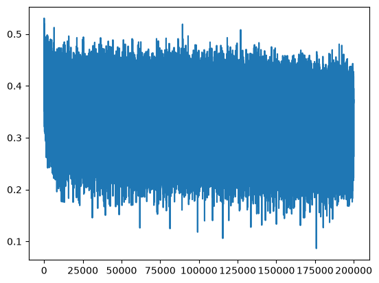

# put layers into evaluation mode (specially needed for batchnorm layer)
for layer in layers:
    layer.training = False

# evaluate the loss
@torch.no_grad() # this decorator disables gradient tracking inside pytorch
def split_loss(split):
  x,y = {
    'train': (Xtr, Ytr),
    'val': (Xdev, Ydev),
    'test': (Xte, Yte),
  }[split]
  emb = C[x] # (N, block_size, n_embd)
  x = emb.view(emb.shape[0], -1) # concat into (N, block_size * n_embd)
  for layer in layers:
    x = layer(x)
  loss = F.cross_entropy(x, y)
  print(split, loss.item())

# put layers into eval mode
for layer in layers:
  layer.training = False
split_loss('train')
split_loss('val')

train 2.058544397354126
val 2.1069703102111816

# validation loss of 2.1069 is fairly good but can be better

# sample from the model

for _ in range(20):

    out = []
    context = [0] * block_size #initialize with all ...

    while True:

        # forward pass the neural net
        emb = C[torch.tensor([context])]   # (1, block_size, n_embd)
        x = emb.view(1, -1)                # (1, block_size*n_embd)
        
        for layer in layers:
            x = layer(x)
        logits = x
        probs = F.softmax(logits, dim=1)

        # sample from the distribution
        ix = torch.multinomial(probs, num_samples=1).item()

        # shift the context window and track the samples
        context = context[1:] + [ix]
        out.append(ix)
        # if we sample the special '.' token, break
        if ix == 0:
            break
        
    print(''.join(itos[i] for i in out)) # decode and print the generated word

noorah.
mit.
shud.
rin.
ristina.
lari.
espinzier.
carkyon.
elyn.
coriah.
sasyleightohalesplenceiomina.
skinnne.
aoryn.
hohby.
miques.
ajan.
kay.
mes.
cael.
crisseie.

plt.plot(lossi)

[<matplotlib.lines.Line2D at 0x7a5194712f90>]

# we'll start by fixing the learning rate plot of lossi
lossi[:10] #list of floats
# we need to average up some of the values to get a more representative value along the way

[0.5193337202072144,
 0.5132609009742737,
 0.5081090927124023,
 0.5117111802101135,
 0.4967299699783325,
 0.4925733506679535,
 0.47202202677726746,
 0.47907018661499023,
 0.48941266536712646,
 0.50093674659729]

# recall
print(torch.arange(10))
print(torch.arange(10).view(2,5))
print(torch.arange(10).view(-1, 2)) #when -1, pytorch estimates the num itself
# basically, it allows us to spread out consecutive values into rows

tensor([0, 1, 2, 3, 4, 5, 6, 7, 8, 9])
tensor([[0, 1, 2, 3, 4],
        [5, 6, 7, 8, 9]])
tensor([[0, 1],
        [2, 3],
        [4, 5],
        [6, 7],
        [8, 9]])

print(torch.tensor(lossi).shape)
print(torch.tensor(lossi).view(-1, 1000).shape) #now we can do a mean along the rows to see the pattern
print(torch.tensor(lossi).view(-1, 1000).mean(1, keepdim=True).shape) #haah, i added keepdim myself
plt.plot(torch.tensor(lossi).view(-1, 1000).mean(1, keepdim=True))

torch.Size([200000])
torch.Size([200, 1000])
torch.Size([200, 1])

[<matplotlib.lines.Line2D at 0x7a519477c2f0>]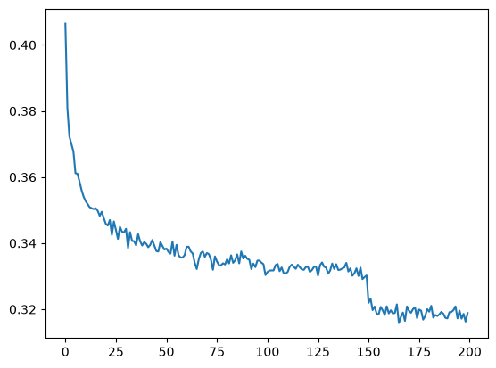

# this graph is a lot better
# the second vertical fall that starts at around x=150 and y=0.33 is the learning rate decay
# learning rate decay allowed us to settle into the local minimum of this optimization

A modular model¶

# next, we fix our code for forward pass to make it more modular and organized
# we organized some layers(eg. linear, etc) inside the layers list but not embedding and viewing operation
# we have this embedding table C and we are indexing at the integers inside batch/tensor XB, 
# so that's an embedding table lookup done with simple indexing
# and the view operation just rearranges the character embeddings and stretches them out into a row
# and it just does the concatenation operation, and its efficient cuz no memory is created/copied, we're just re-representing how we view that tensor
# thus, we create modules for the embedding operation and the flattening operation

# we developed these to mimic the apis of pytorch
class Linear:

    def __init__(self, fan_in, fan_out, bias=True):
        self.weight = torch.randn((fan_in, fan_out)) / fan_in**0.5 #kaiming initialization: look docs
        self.bias = torch.zeros(fan_out) if bias else None

    def __call__(self, x): #its just matrix mul in the forward pass of this module
        self.out = x @ self.weight
        if self.bias is not None:
            self.out += self.bias
        return self.out

    def parameters(self):
        return [self.weight] + ([] if self.bias is None else [self.bias])

class BatchNorm1d:

    def __init__(self, dim, eps=1e-5, momentum = 0.1):
        self.eps = eps
        self.momentum = momentum
        self.training = True #need this flag cuz behaviour of batchnorm is diff during training time and evaluation time, 
        # so need to keep track of state properly, might introduce bugs

        # parameters(trained with backprop)
        self.gamma = torch.ones(dim)
        self.beta = torch.zeros(dim)

        # buffers (trained with a running 'momentum update')
        self.running_mean = torch.zeros(dim)
        self.running_var = torch.ones(dim)

    def __call__(self, x):

        # calculate the forward pass
        if self.training:
            xmean = x.mean(0, keepdim=True) #batch mean
            xvar = x.var(0, keepdim=True) #batch variance
        else:
            xmean = self.running_mean
            xvar = self.running_var

        xhat = (x - xmean) / torch.sqrt(xvar + self.eps) #normalize to unit variance
        self.out = self.gamma * xhat + self.beta

        # update the buffers
        if self.training:
            with torch.no_grad():
                self.running_mean = (1 - self.momentum) * self.running_mean + self.momentum * xmean
                self.running_var = (1 - self.momentum) * self.running_var + self.momentum * xvar
        return self.out

    def parameters(self):
        return [self.gamma, self.beta]

class Tanh:
    def __call__(self, x):
        self.out = torch.tanh(x)
        return self.out

    def parameters(self):
        return []

class Embedding:
    # our lookup table C will become self.weight inside embedding module
    # C = torch.randn((vocab_size, n_embd))
    
    def __init__(self, num_embeddings, embedding_dim):
        self.weight = torch.randn(num_embeddings, embedding_dim)

    def __call__(self, IX):
        self.out = self.weight[IX] #indexing operation in forward pass
        return self.out

    def parameters(self):
        return [self.weight]

class Flatten:
    def __call__(self, x):
        self.out = x.view(x.shape[0], -1) #flattening operation in forward pass
        return self.out

    def parameters(self):
        return []

# these Embedding, Flatten also exist in pytorch

n_embd = 10 #dimensionality of character embedding vectors
n_hidden = 200 #number of neurons in hidden layer of MLP

# C = torch.randn((vocab_size, n_embd)) #notice there's no generator g
layers = [
    Embedding(vocab_size, n_embd), #initializes C
    Flatten(),
    Linear(n_embd * block_size, n_hidden, bias=False), 
    BatchNorm1d(n_hidden), 
    Tanh(),
    Linear(n_hidden, vocab_size),
]

with torch.no_grad():
    layers[-1].weight *= 0.1 # make last layer less confident, so we're not confidently wrong at initialization

# parameter initialization
# parameters = [C] + [p for layer in layers for p in layer.parameters()]
parameters = [p for layer in layers for p in layer.parameters()] #removed C cuz it's now inside layers list above
print(sum(p.nelement() for p in parameters)) # no of parameters in total
for p in parameters:
    p.requires_grad = True

# same optimization as previously done
max_steps = 200000
batch_size = 32
lossi = []

for i in range(max_steps):

    # minibatch construct
    ix = torch.randint(0, Xtr.shape[0], (batch_size, ))
    Xb, Yb = Xtr[ix], Ytr[ix] #batch X, Y

    # forward pass
    # emb = C[Xb] #embed the characters into vectors
    # x = emb.view(emb.shape[0], -1) #concatenate the vectors
    x = Xb #to kick things off in the beginning, x=X=tensor of integers specifying the identities of these characters at the input, and we feed these chars to the layer
    for layer in layers:
        x = layer(x)
    loss = F.cross_entropy(x, Yb) #loss function

    # # backward pass
    for p in parameters:
        p.grad = None
    loss.backward()

    # update: simple SGD
    lr = 0.1 if i < 150000 else 0.01 # step learning rate decay
    for p in parameters:
        p.data += -lr * p.grad

    # track stats
    if i % 10000 == 0: #print every once in a while
        print(f'{i:7d}/{max_steps:7d}: {loss.item():.4f}')
    lossi.append(loss.log10().item())

    break

      0/ 200000: 3.2924

# next improvement: 
# currently, we are maintaining all of our modules in a naked list of layers, and we want to simplify this as well
# we introduce the concept of pytorch containers in torch.nn
# containers are basically a way of organizing layers into lists/dicts/etc
# there is something called "sequential" inside containers which maintains a list of layers, and is a module class in pytorch
# and it just passes a given input through all the layers sequentially exactly as we're doing here, lets write our own sequential
# o/p of one will be i/p to next, and so on until end

https://docs.pytorch.org/docs/2.13/generated/torch.nn.Sequential.html

# we developed these to mimic the apis of pytorch
class Linear:

    def __init__(self, fan_in, fan_out, bias=True):
        self.weight = torch.randn((fan_in, fan_out)) / fan_in**0.5 #kaiming initialization: look docs, #weight is 2-dimensional
        self.bias = torch.zeros(fan_out) if bias else None #bias is 1-dimensional

    def __call__(self, x): #its just matrix mul in the forward pass of this module
        # the linear layer takes input x, multiplies it with weight and optionally adds bias: i.e. wx + b
        self.out = x @ self.weight
        if self.bias is not None:
            self.out += self.bias
        return self.out

    def parameters(self):
        return [self.weight] + ([] if self.bias is None else [self.bias])

class BatchNorm1d:

    def __init__(self, dim, eps=1e-5, momentum = 0.1):
        self.eps = eps
        self.momentum = momentum
        self.training = True #need this flag cuz behaviour of batchnorm is diff during training time and evaluation time, 
        # so need to keep track of state properly, might introduce bugs

        # parameters(trained with backprop)
        self.gamma = torch.ones(dim)
        self.beta = torch.zeros(dim)

        # buffers (trained with a running 'momentum update')
        self.running_mean = torch.zeros(dim)
        self.running_var = torch.ones(dim)

    def __call__(self, x):

        # calculate the forward pass
        if self.training:
            xmean = x.mean(0, keepdim=True) #batch mean
            xvar = x.var(0, keepdim=True) #batch variance
        else:
            xmean = self.running_mean
            xvar = self.running_var

        xhat = (x - xmean) / torch.sqrt(xvar + self.eps) #normalize to unit variance
        self.out = self.gamma * xhat + self.beta

        # update the buffers
        if self.training:
            with torch.no_grad():
                self.running_mean = (1 - self.momentum) * self.running_mean + self.momentum * xmean
                self.running_var = (1 - self.momentum) * self.running_var + self.momentum * xvar
        return self.out

    def parameters(self):
        return [self.gamma, self.beta]

class Tanh:
    def __call__(self, x):
        self.out = torch.tanh(x)
        return self.out

    def parameters(self):
        return []

class Embedding:
    # our lookup table C will become self.weight inside embedding module
    # C = torch.randn((vocab_size, n_embd))
    
    def __init__(self, num_embeddings, embedding_dim):
        self.weight = torch.randn(num_embeddings, embedding_dim)

    def __call__(self, IX):
        self.out = self.weight[IX] #indexing operation in forward pass
        return self.out

    def parameters(self):
        return [self.weight]

class Flatten:
    def __call__(self, x):
        self.out = x.view(x.shape[0], -1) #flattening operation in forward pass
        return self.out

    def parameters(self):
        return []

class Sequential:
    # pass in our list of layers
    def __init__(self, layers):
        self.layers = layers

    # for any input in forward pass, call the layers sequentialy as before
    def __call__(self, x):
        for layer in self.layers:
            x = layer(x)
        self.out = x
        return self.out

    def parameters(self):
        # get parameters of all layers and stretch them out into one list
        return [p for layer in self.layers for p in layer.parameters()]

torch.manual_seed(42);

n_embd = 10 #dimensionality of character embedding vectors
n_hidden = 200 #number of neurons in hidden layer of MLP

# C = torch.randn((vocab_size, n_embd)) #notice there's no generator g
# we no longer maintain a naked list of layers, instead we use a module
# layers = [
#     Embedding(vocab_size, n_embd), #initializes C
#     Flatten(),
#     Linear(n_embd * block_size, n_hidden, bias=False), 
#     BatchNorm1d(n_hidden), 
#     Tanh(),
#     Linear(n_hidden, vocab_size),
# ]
model = Sequential([
        Embedding(vocab_size, n_embd), #initializes C
        Flatten(),
        Linear(n_embd * block_size, n_hidden, bias=False), 
        BatchNorm1d(n_hidden), 
        Tanh(),
        Linear(n_hidden, vocab_size),
])

with torch.no_grad():
    layers[-1].weight *= 0.1 # make last layer less confident, so we're not confidently wrong at initialization

# parameter initialization
# parameters = [C] + [p for layer in layers for p in layer.parameters()]
# parameters = [p for layer in layers for p in layer.parameters()] #this logic lives inside Sequential
parameters = model.parameters()
print(sum(p.nelement() for p in parameters)) # no of parameters in total
for p in parameters:
    p.requires_grad = True

# had 12097 parameters when block_size was 3

# same optimization as previously done
max_steps = 200000
batch_size = 32
lossi = []

for i in range(max_steps):

    # minibatch construct
    ix = torch.randint(0, Xtr.shape[0], (batch_size, ))
    Xb, Yb = Xtr[ix], Ytr[ix] #batch X, Y

    # forward pass
    # no need to do forward pass here, we just call the model on the input data, 
    # x = Xb
    # for layer in layers:
    #     x = layer(x)

    logits = model(Xb)
    loss = F.cross_entropy(logits, Yb) #loss function takes the logits and the targets

    # # backward pass
    for p in parameters:
        p.grad = None
    loss.backward()

    # update: simple SGD
    lr = 0.1 if i < 150000 else 0.01 # step learning rate decay
    for p in parameters:
        p.data += -lr * p.grad

    # track stats
    if i % 10000 == 0: #print every once in a while
        print(f'{i:7d}/{max_steps:7d}: {loss.item():.4f}')
    lossi.append(loss.log10().item())

    # break

      0/ 200000: 3.5336
  10000/ 200000: 2.3646
  20000/ 200000: 2.4790
  30000/ 200000: 2.2761
  40000/ 200000: 2.0539
  50000/ 200000: 2.5657
  60000/ 200000: 2.5574
  70000/ 200000: 1.8780
  80000/ 200000: 1.8933
  90000/ 200000: 1.6215
 100000/ 200000: 2.3156
 110000/ 200000: 2.1761
 120000/ 200000: 2.0617
 130000/ 200000: 2.0571
 140000/ 200000: 2.5551
 150000/ 200000: 2.1006
 160000/ 200000: 1.9694
 170000/ 200000: 2.2940
 180000/ 200000: 2.2346
 190000/ 200000: 1.9638

# same optimization as previously done but for block_size: 8
max_steps = 200000
batch_size = 32
lossi = []

for i in range(max_steps):

    # minibatch construct
    ix = torch.randint(0, Xtr.shape[0], (batch_size, ))
    Xb, Yb = Xtr[ix], Ytr[ix] #batch X, Y

    # forward pass
    # no need to do forward pass here, we just call the model on the input data, 
    # x = Xb
    # for layer in layers:
    #     x = layer(x)

    logits = model(Xb)
    loss = F.cross_entropy(logits, Yb) #loss function takes the logits and the targets

    # # backward pass
    for p in parameters:
        p.grad = None
    loss.backward()

    # update: simple SGD
    lr = 0.1 if i < 150000 else 0.01 # step learning rate decay
    for p in parameters:
        p.data += -lr * p.grad

    # track stats
    if i % 10000 == 0: #print every once in a while
        print(f'{i:7d}/{max_steps:7d}: {loss.item():.4f}')
    lossi.append(loss.log10().item())

    # break

      0/ 200000: 3.5614
  10000/ 200000: 2.0009
  20000/ 200000: 1.9863
  30000/ 200000: 2.4963
  40000/ 200000: 2.2945
  50000/ 200000: 2.2080
  60000/ 200000: 2.3371
  70000/ 200000: 1.7947
  80000/ 200000: 1.9881
  90000/ 200000: 2.2709
 100000/ 200000: 2.4245
 110000/ 200000: 1.9647
 120000/ 200000: 2.0879
 130000/ 200000: 2.2980
 140000/ 200000: 2.5866
 150000/ 200000: 1.9837
 160000/ 200000: 1.8209
 170000/ 200000: 1.8292
 180000/ 200000: 2.0675
 190000/ 200000: 2.0119

# put layers into evaluation mode (specially needed for batchnorm layer)
for layer in model.layers:
    layer.training = False

# if you forget to run the cell to set layer.training=False after training, and when you want to test
# you'll get error or incorrect results
# eg. in test, we are passing an input which is a batch of just a single example 
# and if we pass just a single example into batchnorm in training mode, you'll estimate the variance using the input
# and the variance of a single number is nan cuz variance/s.d. is a measure of the spread
# and we won't see the issue with loss, it will be evaluated but give the wrong result cuz batchnorm is still in traning mode if that cell above is not run
# cuz in testing, it will use the sample statistics of batch whereas we want to use the runningmean and runningvar inside batchnorm
# thus, if you don't maintain state properly, you'll get bug

# example: variance of a single number is nan
torch.var(torch.tensor([8.0]))

/tmp/ipykernel_47933/2552686865.py:2: UserWarning: var(): degrees of freedom is <= 0. Correction should be strictly less than the reduction factor (input numel divided by output numel). (Triggered internally at /pytorch/aten/src/ATen/native/ReduceOps.cpp:1879.)
  torch.var(torch.tensor([8.0]))

tensor(nan)

# evaluate the loss
@torch.no_grad() # this decorator disables gradient tracking inside pytorch
def split_loss(split):
  x,y = {
    'train': (Xtr, Ytr),
    'val': (Xdev, Ydev),
    'test': (Xte, Yte),
  }[split]

  logits = model(x)
  # emb = C[x] # (N, block_size, n_embd)
  # x = emb.view(emb.shape[0], -1) # concat into (N, block_size * n_embd)
  # for layer in layers:
  #   x = layer(x)
  loss = F.cross_entropy(logits, y)
  print(split, loss.item())

# put layers into eval mode
for layer in layers:
  layer.training = False
split_loss('train')
split_loss('val')
# currently ran only 1 iteration so very high

train 1.9230281114578247
val 2.0320310592651367

# sample from the model

for _ in range(20):

    out = []
    context = [0] * block_size #initialize with all ...

    while True:

        # forward pass the neural net
        logits = model(torch.tensor([context]))
        
        # # forward pass the neural net
        # emb = C[torch.tensor([context])]   # (1, block_size, n_embd)
        # x = emb.view(1, -1)                # (1, block_size*n_embd)
        
        # for layer in layers:
        #     x = layer(x)
        # logits = x
        probs = F.softmax(logits, dim=1)

        # sample from the distribution
        ix = torch.multinomial(probs, num_samples=1).item()

        # shift the context window and track the samples
        context = context[1:] + [ix]
        out.append(ix)
        # if we sample the special '.' token, break
        if ix == 0:
            break
        
    print(''.join(itos[i] for i in out)) # decode and print the generated word
# so the op is trash cuz we trained our model for only 1 iteration
# and op is fine if trained for lots of iterations

ivya.
fadily.
thio.
masan.
emo.
maayannessa.
gaverley.
danaiif.
jazum.
carleon.
jir.
joan.
galoniiah.
jas.
vishylaharian.
daravio.
orven.
mickela.
leigh.
zeffeaustyla.

# sample from the model

for _ in range(20):

    out = []
    context = [0] * block_size #initialize with all ...

    while True:

        # forward pass the neural net
        logits = model(torch.tensor([context]))
        
        # # forward pass the neural net
        # emb = C[torch.tensor([context])]   # (1, block_size, n_embd)
        # x = emb.view(1, -1)                # (1, block_size*n_embd)
        
        # for layer in layers:
        #     x = layer(x)
        # logits = x
        probs = F.softmax(logits, dim=1)

        # sample from the distribution
        ix = torch.multinomial(probs, num_samples=1).item()

        # shift the context window and track the samples
        context = context[1:] + [ix]
        out.append(ix)
        # if we sample the special '.' token, break
        if ix == 0:
            break
        
    print(''.join(itos[i] for i in out)) # decode and print the generated word

melar.
lyri.
gwosen.
darryn.
zakayah.
elsha.
taliyana.
jayah.
ziyah.
hamilinse.
chann.
shadualee.
aladay.
maceel.
hamby.
dweon.
suhaya.
kaylin.
covranni.
gitir.

Comparing context lengths¶

# 3 character context:
train 2.0593066215515137
val 2.1068434715270996

8 character context:
train 1.9230281114578247
val 2.0320310592651367

# since these 2 losses are very similar to each other, we have a sense that they're not overfitting too much 
# and we can make additional progress in our performance by scaling up the size of the neural network 
# in our current architecture, we are taking some characters (3) going into a single hidden layer, then going to prediction of next character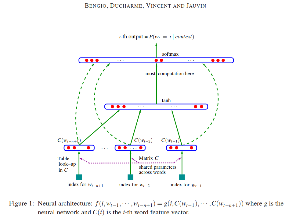

Open original image: ithwordneuralarch.png

# the problem with this: we can't make this bigger in a productive way
# cuz we're crushing all characters into a single layer all the way at the beginning
# and even if we make it bigger by eg. adding neurons, its still silly to squash all that info fast in a single step
# so we'd want our network to look more like the following in the wavenet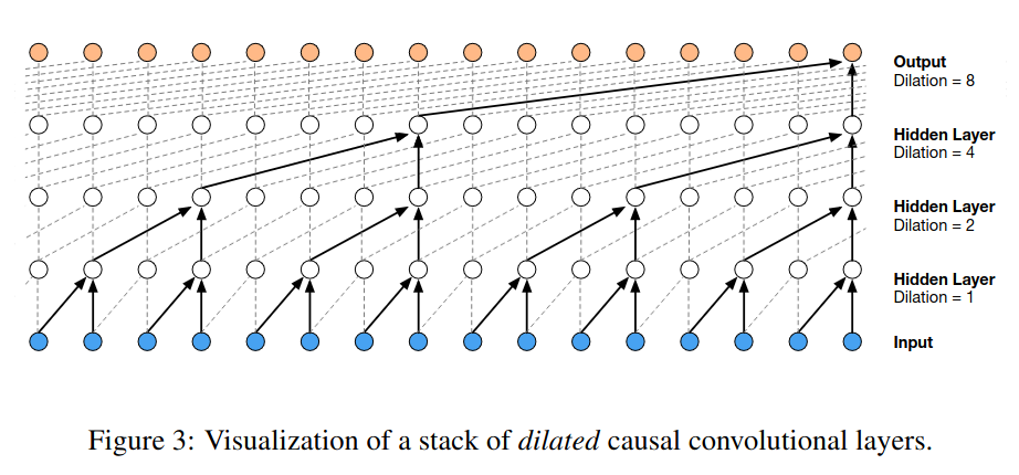

https://arxiv.org/pdf/1609.03499

Open original image: wavenetdilutedlayers.png

Progressively combining characters¶

# Problem with the current architecture:
# - All characters are crushed into a single layer very early.
# - Even making this layer wider still squashes too much information at once.

# WaveNet-style idea:
# - Preserve information longer by progressively combining the context.
# - Fuse 2 characters → bigram representation.
# - Fuse 2 bigrams → 4-character representation.
# - Fuse 2 four-grams → 8-character representation.
# - Continue this in a tree-like, hierarchical manner.

# This creates a deeper network where context is gradually fused as we go deeper.
# In WaveNet, this is implemented using dilated causal convolution layers.
# "Dilated" and "causal" are mainly implementation details for efficiency;
# the key idea to understand is PROGRESSIVE FUSION.

# Goal:
# - Build a deeper architecture that progressively fuses:
#   characters → bigrams → 4-grams → 8-grams → ...
# - At each level, fuse only two consecutive elements.

# upon increasing context length / block_size from 3 to 8, and running it without any change, there was significant improvement in loss as you can see above
# it increases no of parameters obviously
# continue from 21:35

# lets look at the forward pass of the neural net and 
# inspect the shape of the tensor along the way as the neural net forwards
# lets look at a batch of 4 examples
ix = torch.randint(0, Xtr.shape[0], (4, ))
Xb, Yb = Xtr[ix], Ytr[ix] #pluck out rows from our training set
logits = model(Xb)
print(Xb.shape) #4 examples(each row of Xb) x block size = 8, i.e. 8 integers for a character as context
Xb

torch.Size([4, 8])

tensor([[ 0,  0,  0, 11,  1, 13, 18, 25],
        [ 0,  0,  0,  0,  0, 25,  1, 14],
        [ 0,  0,  0,  0,  0,  0,  0, 20],
        [ 0,  0,  0,  0,  2,  5,  3, 11]])

# passing Xb through the embedding layer creates output of shape 4x8x10
# embedding layer plucks out the embedding vector and organizes each of the 8 integers into a 10 dimensional vector
model.layers[0].out.shape #output of embedding layer

torch.Size([4, 8, 10])

# stretch out 8x10 into a single row, we view it differently, by concatenation
model.layers[1].out.shape #output of flatten layer

torch.Size([4, 80])

model.layers[2].out.shape #output of linear layer, takes in 80 and creates 200 channels via matrix multiplication

torch.Size([4, 200])

# what's happening inside this linear layer looks like this
# xw + b, the shape of the matrix that comes out of linear layer is 4x200
(torch.randn(4, 80) @ torch.randn(80, 200) + torch.randn(200)).shape
# there is broadcasting here: 4x200 + 200 -> 4x200 + 1x200, then this 1x200 replicates to be 4x200, its okay

torch.Size([4, 200])

# surprising thing is that this input X being multiplied with weight matrix W doesn't have to be 2-dimensional 
# the matrix multiplication operator @ is quite powerful, so you can pass higher dimensional arrays/tensors
# example:
(torch.randn(4, 5, 2, 80) @ torch.randn(80, 200) + torch.randn(200)).shape

torch.Size([4, 5, 2, 200])

# what happens here is that matrix mul works on the last dimension only, and previous dimensions remain unchanged
# and we can use this on our network now

# remember that we have 8 characters coming in: 1 2 3 4 5 6 7 8 and 
# we don't want to flatten all of it out into a large eight-dimensional vector: remember concept of wavenet
# we want to group it like this: (1 2) (3 4) (5 6) (7 8), we want to create four sub groups and process these bigram groups in parallel
# we don't want 8 characters coming in all at once, 
# we want 2 characters coming in on the first layer, and these 2 characters should be fused
# so we don't want (ax8) x (8xb), we want (a x 4 x 2) x (2 x b)

# (torch.randn(4, 80) @ torch.randn(80, 200) + torch.randn(200)).shape
# (torch.randn(4, 4, 20) @ torch.randn(20, 200) + torch.randn(200)).shape is what we want
# but to do this, we want the flatten layer to also output (4, 4, 20) instead of (4, 80)
# just pack in every 2 consecutive characters on the last dimension

# so we have to change Linear layer: should expect 20 instead of 80
# also, we have to change Flatten layer: should output (4, 4, 20) instead of (4, 80)

model.layers[0].out.shape #output of embedding layer, want this to be 4,4,20 instead

torch.Size([4, 8, 10])

# modify our flatten layer code, currently it does: self.out = x.view(x.shape[0], -1)

print(list(range(10)))
print(list(range(10))[:])
print(list(range(10))[::])
print(list(range(10))[1::]) #initial part is start num
print(list(range(10))[::2]) #later part is called slice step
print(list(range(10))[::5])

[0, 1, 2, 3, 4, 5, 6, 7, 8, 9]
[0, 1, 2, 3, 4, 5, 6, 7, 8, 9]
[0, 1, 2, 3, 4, 5, 6, 7, 8, 9]
[1, 2, 3, 4, 5, 6, 7, 8, 9]
[0, 2, 4, 6, 8]
[0, 5]

print(list(range(10))[1::2]) #get all odd parts
print(list(range(10))[::2]) #get all even parts

[1, 3, 5, 7, 9]
[0, 2, 4, 6, 8]

e = torch.randn(4, 8, 10) #4x8x10 matrix, want this to be 4x4x20 matrix

# for all batch elements in first dimension, only even elements in second dimension, i.e. at indexes 0,2,4,6,8, and for all parts in last dimension
# first one gives even characters, second one gives odd characters, we want to concatenate these tensors along second dimension
e[:, ::2, :], e[:, 1::2, :]
explicit_concat = torch.cat([e[:, ::2, :], e[:, 1::2, :]], dim=2) # yes this shape is exactly what we want
# we're gathering these even parts and odd parts eg. (0,1) and arranging each of these 4x4x10 and concatenating them to make 4x4x20
explicit_concat.shape

torch.Size([4, 4, 20])

# this works but what also works is by using view to request right shape, and it is what we expect
e.view(4,4,20) == explicit_concat
(e.view(4,4,20) == explicit_concat).all()

tensor(True)

# so no need to make explicit call to torch.cat, i.e. concatenate, we can just take input tensor and view it in whatever way we want
# we don't want to stretch things out with -1, we want to create 3d array, fuse eg. 2 consecutive vectors and ask dimension

# torch.squeeze: Returns a tensor with all specified dimensions of input of size 1 removed.
# For example, if input is of shape: (A×1×B×C×1×D)(A×1×B×C×1×D) then the input.squeeze() will be of shape: (A×B×C×D)(A×B×C×D).
# When dim is given, a squeeze operation is done only in the given dimension(s). If input is of shape: (A×1×B)(A×1×B), 
# squeeze(input, 0) leaves the tensor unchanged, but squeeze(input, 1) will squeeze the tensor to the shape (A×B)(A×B).

Grouping and flattening¶

# pytorch also has a Flatten but its keyword arguments are different, but ours will be different so naming different
# flattens some n consecutive elements and puts them into last dimension
class FlattenConsecutive:
    
    def __init__(self, n):
        self.n = n

    def __call__(self, x):
        B, T, C = x.shape #eg. 4x8x10
        # x = x.view(B, -1, C*n) #-1 means pytorch will figure it out itself, n=how many consecutive elements we want eg. 2 for (1,2) (3,4) (5,6)
        x = x.view(B, T//self.n, C*self.n) # //: integer division
        # though -1 should work fine, we want to be explicit in keeping shape cuz we get error messages when things don't go acc to our expectations

        # remember in the very beginning, n=3 and we concatenated all 3 chars, so sometimes we want a fake dimension of 1 in middle, an exceptional case
        if(x.shape[1] == 1): #return a 2d tensor as we did before: self.out = x.view(x.shape[0], -1)
            x = x.squeeze(1) # so if input is B x 1 x C, we want to return 2d tensor B x C*n

        self.out = x
        return self.out

    def parameters(self):
        return []

n_embd = 10 #dimensionality of character embedding vectors
n_hidden = 200 #number of neurons in hidden layer of MLP

model = Sequential([
        Embedding(vocab_size, n_embd), #initializes C
        # Flatten(),
        FlattenConsecutive(block_size),
        Linear(n_embd * block_size, n_hidden, bias=False), 
        BatchNorm1d(n_hidden), 
        Tanh(),
        Linear(n_hidden, vocab_size),
])

with torch.no_grad():
    layers[-1].weight *= 0.1 # make last layer less confident, so we're not confidently wrong at initialization

# parameter initialization
# parameters = [C] + [p for layer in layers for p in layer.parameters()]
# parameters = [p for layer in layers for p in layer.parameters()] #this logic lives inside Sequential
parameters = model.parameters()
print(sum(p.nelement() for p in parameters)) # no of parameters in total
for p in parameters:
    p.requires_grad = True

# had 12097 parameters when block_size was 3

ix = torch.randint(0, Xtr.shape[0], (4, ))
Xb, Yb = Xtr[ix], Ytr[ix] #pluck out rows from our training set
logits = model(Xb)
print(Xb.shape) #4 examples(each row of Xb) x block size = 8, i.e. 8 integers for a character as context
Xb

torch.Size([4, 8])

tensor([[ 0,  0,  0,  0,  0, 13,  1, 18],
        [ 0,  0,  0,  8,  1, 12,  5,  5],
        [ 0,  0,  0,  1, 13,  2,  5, 18],
        [ 0,  0,  0, 19,  8,  1, 11, 25]])

for layer in model.layers:
    print(layer.__class__.__name__, ':', tuple(layer.out.shape))

Embedding : (4, 8, 10)
FlattenConsecutive : (4, 80)
Linear : (4, 200)
BatchNorm1d : (4, 200)
Tanh : (4, 200)
Linear : (4, 27)

# now we achieve what we want to

n_embd = 10 #dimensionality of character embedding vectors
n_hidden = 200 #number of neurons in hidden layer of MLP

model = Sequential([
        Embedding(vocab_size, n_embd), #initializes C
        FlattenConsecutive(2), Linear(n_embd * 2, n_hidden, bias=False), BatchNorm1d(n_hidden), Tanh(),
        FlattenConsecutive(2), Linear(n_hidden * 2, n_hidden, bias=False), BatchNorm1d(n_hidden), Tanh(),
        FlattenConsecutive(2), Linear(n_hidden * 2, n_hidden, bias=False), BatchNorm1d(n_hidden), Tanh(),
        Linear(n_hidden, vocab_size),
])

with torch.no_grad():
    layers[-1].weight *= 0.1 # make last layer less confident, so we're not confidently wrong at initialization

# parameter initialization
# parameters = [C] + [p for layer in layers for p in layer.parameters()]
# parameters = [p for layer in layers for p in layer.parameters()] #this logic lives inside Sequential
parameters = model.parameters()
print(sum(p.nelement() for p in parameters)) # no of parameters in total
for p in parameters:
    p.requires_grad = True

# had 22097 parameters

ix = torch.randint(0, Xtr.shape[0], (4, ))
Xb, Yb = Xtr[ix], Ytr[ix] #pluck out rows from our training set
logits = model(Xb)
print(Xb.shape) #4 examples(each row of Xb) x block size = 8, i.e. 8 integers for a character as context
Xb

torch.Size([4, 8])

tensor([[ 0,  0,  0,  0,  0,  0,  8, 21],
        [ 0,  0,  0,  0,  0,  0,  0,  1],
        [ 0,  0,  0,  0,  0,  0,  1,  2],
        [ 5,  4,  4,  9, 14,  7, 20, 15]])

for layer in model.layers:
    print(layer.__class__.__name__, ':', tuple(layer.out.shape))

# notice the last flatten consecutive squeezed out the dimension of 1

Embedding : (4, 8, 10)
FlattenConsecutive : (4, 4, 20)
Linear : (4, 4, 200)
BatchNorm1d : (4, 4, 200)
Tanh : (4, 4, 200)
FlattenConsecutive : (4, 2, 400)
Linear : (4, 2, 200)
BatchNorm1d : (4, 2, 200)
Tanh : (4, 2, 200)
FlattenConsecutive : (4, 400)
Linear : (4, 200)
BatchNorm1d : (4, 200)
Tanh : (4, 200)
Linear : (4, 27)

logits.shape #logits are in the same shape as before, but now our neural net has 3 layers

torch.Size([4, 27])

# our network now corresponds to this: blocksize = 8, layercount = 3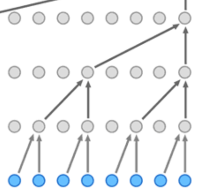

Open original image: wavenet3layers8inputs.png

# now we chose n_hidden = 68, because its about the same parameters as before: approx 20,000, we want to compare performance increase by use of wavenet
# rather than just improve loss cuz we're learning ofcourse
# we want to see if the parameters are utilized in a more efficient architecture

n_embd = 10 #dimensionality of character embedding vectors
n_hidden = 68 #number of neurons in hidden layer of MLP

model = Sequential([
        Embedding(vocab_size, n_embd), #initializes C
        FlattenConsecutive(2), Linear(n_embd * 2, n_hidden, bias=False), BatchNorm1d(n_hidden), Tanh(),
        FlattenConsecutive(2), Linear(n_hidden * 2, n_hidden, bias=False), BatchNorm1d(n_hidden), Tanh(),
        FlattenConsecutive(2), Linear(n_hidden * 2, n_hidden, bias=False), BatchNorm1d(n_hidden), Tanh(),
        Linear(n_hidden, vocab_size),
])

with torch.no_grad():
    layers[-1].weight *= 0.1 # make last layer less confident, so we're not confidently wrong at initialization

# parameter initialization
# parameters = [C] + [p for layer in layers for p in layer.parameters()]
# parameters = [p for layer in layers for p in layer.parameters()] #this logic lives inside Sequential
parameters = model.parameters()
print(sum(p.nelement() for p in parameters)) # no of parameters in total
for p in parameters:
    p.requires_grad = True

# had 22097 parameters

# put layers into evaluation mode: needed for batchnorm layer
for layer in model.layers:
    layer.training = False

# evaluate the loss
@torch.no_grad() # this decorator disables gradient tracking inside pytorch
def split_loss(split):
  x,y = {
    'train': (Xtr, Ytr),
    'val': (Xdev, Ydev),
    'test': (Xte, Yte),
  }[split]

  logits = model(x)
  loss = F.cross_entropy(logits, y)
  print(split, loss.item())

split_loss('train')
split_loss('val')
# currently ran only 1 iteration so very high

train 3.471845865249634
val 3.4728987216949463

Training the hierarchy¶

# same optimization as previously done but for block_size: 8
max_steps = 200000
batch_size = 32
lossi = []

for i in range(max_steps):

    # minibatch construct
    ix = torch.randint(0, Xtr.shape[0], (batch_size, ))
    Xb, Yb = Xtr[ix], Ytr[ix] #batch X, Y

    # forward pass
    logits = model(Xb)
    loss = F.cross_entropy(logits, Yb) #loss function takes the logits and the targets

    # # backward pass
    for p in parameters:
        p.grad = None
    loss.backward()

    # update: simple SGD
    lr = 0.1 if i < 150000 else 0.01 # step learning rate decay
    for p in parameters:
        p.data += -lr * p.grad

    # track stats
    if i % 10000 == 0: #print every once in a while
        print(f'{i:7d}/{max_steps:7d}: {loss.item():.4f}')
    lossi.append(loss.log10().item())

    break

      0/ 200000: 2.0666

# even running for 200,000 iterations, there wasn't much difference
# we found that there was not much difference cuz a bug exists in batchnorm layer, lets fix it first then train our model finally

for layer in model.layers:
    print(layer.__class__.__name__, ':', tuple(layer.out.shape))

Embedding : (22767, 8, 10)
FlattenConsecutive : (22767, 4, 20)
Linear : (22767, 4, 68)
BatchNorm1d : (22767, 4, 68)
Tanh : (22767, 4, 68)
FlattenConsecutive : (22767, 2, 136)
Linear : (22767, 2, 68)
BatchNorm1d : (22767, 2, 68)
Tanh : (22767, 2, 68)
FlattenConsecutive : (22767, 136)
Linear : (22767, 68)
BatchNorm1d : (22767, 68)
Tanh : (22767, 68)
Linear : (22767, 27)

# look here, batchnorm receives input tensor of shape axbxc:
# Linear : (22767, 4, 68)
# BatchNorm1d : (22767, 4, 68)
# at the time we wrote batchnorm, we assumed that x is 2 dimensional (batch_size x d)
# so we reduced the mean and the variance over the 0th dimension as x.mean(0), x.var(0)
# though there are a dimensions, we're doing mean only over the 0th dimension
# then why's batchnorm working and not getting any errors?: cuz everything broadcast properly, but not how we want it to

# # inside class BatchNorm1d:
#  def __call__(self, x):

#         # calculate the forward pass
#         if self.training:
#             xmean = x.mean(0, keepdim=True) #batch mean
#             xvar = x.var(0, keepdim=True) #batch variance
#         else:
#             xmean = self.running_mean
#             xvar = self.running_var

#         xhat = (x - xmean) / torch.sqrt(xvar + self.eps) #normalize to unit variance
#         self.out = self.gamma * xhat + self.beta

#         # update the buffers
#         if self.training:
#             with torch.no_grad():
#                 self.running_mean = (1 - self.momentum) * self.running_mean + self.momentum * xmean
#                 self.running_var = (1 - self.momentum) * self.running_var + self.momentum * xvar
#         return self.out

Diagnosing the normalization dimensions¶

# what went wrong:
e = torch.randn(22767, 4, 68)
emean = e.mean(0, keepdim=True) # 1 x 4 x 68, i.e. only processes mean for one out of 22k+ dimensions
evar = e.var(0, keepdim=True) # 1 x 4 x 68
ehat = (e - emean) / torch.sqrt(evar + 1e-5) #22767 x 4 x 68: works out cuz of broadcasting
ehat.shape

torch.Size([22767, 4, 68])

# look at running mean shape confirms this too
model.layers[3].running_mean.shape

# we want to treat that 4 as a batch dimension like the 0th dimension
# we don't want to average over 22767 numbers, but average over 22767 x 4 numbers for every single one of 68 channels

torch.Size([1, 4, 68])

# look at docs of torch.mean
# parameters: dim (int or tuple of ints, optional) – the dimension or dimensions to reduce. If None, all dimensions are reduced.
# we can pass a tuple instead of single dimension

https://docs.pytorch.org/docs/2.13/generated/torch.mean.html

# fix is pretty simple, just include both dimensions
#  def __call__(self, x):

#         # calculate the forward pass
#         if self.training:
                # if x.ndim == 2:
                #     dim = 0 #same as prev
                # elif x.ndim == 3:
                #     dim = (0,1)
                # and we get error for other dim tensor, which is good
    #             xmean = x.mean(dim, keepdim=True) #batch mean
    #             xvar = x.var(dim, keepdim=True) #batch variance
# but here, we're departing from api of pytorch by a little, pytorch's takes both 2 and 3 dimension as input
# pytorch assumes no of channels will always be in middle i.e. first dimension, but we're assuming it to be in last dimension eg. 1 or 2
# and some batch dimension occur beforehand
# pytorch expects (N, C) or (N, C, L)
# we expect (N, C) or (N, L, C)
# N=batch size, C=no of channels, L=sequence length

# now our complete changes

class Linear:

    def __init__(self, fan_in, fan_out, bias=True):
        self.weight = torch.randn((fan_in, fan_out)) / fan_in**0.5 #kaiming initialization: look docs, #weight is 2-dimensional
        self.bias = torch.zeros(fan_out) if bias else None #bias is 1-dimensional

    def __call__(self, x): #its just matrix mul in the forward pass of this module
        # the linear layer takes input x, multiplies it with weight and optionally adds bias: i.e. wx + b
        self.out = x @ self.weight
        if self.bias is not None:
            self.out += self.bias
        return self.out

    def parameters(self):
        return [self.weight] + ([] if self.bias is None else [self.bias])

class BatchNorm1d:

    def __init__(self, dim, eps=1e-5, momentum = 0.1):
        self.eps = eps
        self.momentum = momentum
        self.training = True #need this flag cuz behaviour of batchnorm is diff during training time and evaluation time, 
        # so need to keep track of state properly, might introduce bugs

        # parameters(trained with backprop)
        self.gamma = torch.ones(dim)
        self.beta = torch.zeros(dim)

        # buffers (trained with a running 'momentum update')
        self.running_mean = torch.zeros(dim)
        self.running_var = torch.ones(dim)

    def __call__(self, x):

        # calculate the forward pass
        if self.training:
            if x.ndim == 2:
                    dim = 0 #same as prev
            elif x.ndim == 3:
                    dim = (0,1)
        # and we get error for other dim tensor, which is good
            xmean = x.mean(dim, keepdim=True) #batch mean
            xvar = x.var(dim, keepdim=True) #batch variance
        else:
            xmean = self.running_mean
            xvar = self.running_var

        xhat = (x - xmean) / torch.sqrt(xvar + self.eps) #normalize to unit variance
        self.out = self.gamma * xhat + self.beta

        # update the buffers
        if self.training:
            with torch.no_grad():
                self.running_mean = (1 - self.momentum) * self.running_mean + self.momentum * xmean
                self.running_var = (1 - self.momentum) * self.running_var + self.momentum * xvar
        return self.out

    def parameters(self):
        return [self.gamma, self.beta]

class Tanh:
    def __call__(self, x):
        self.out = torch.tanh(x)
        return self.out

    def parameters(self):
        return []

class Embedding:
    # our lookup table C will become self.weight inside embedding module
    # C = torch.randn((vocab_size, n_embd))
    
    def __init__(self, num_embeddings, embedding_dim):
        self.weight = torch.randn(num_embeddings, embedding_dim)

    def __call__(self, IX):
        self.out = self.weight[IX] #indexing operation in forward pass
        return self.out

    def parameters(self):
        return [self.weight]

class FlattenConsecutive:
    
    def __init__(self, n):
        self.n = n

    def __call__(self, x):
        B, T, C = x.shape #eg. 4x8x10
        # x = x.view(B, -1, C*n) #-1 means pytorch will figure it out itself, n=how many consecutive elements we want eg. 2 for (1,2) (3,4) (5,6)
        x = x.view(B, T//self.n, C*self.n) # //: integer division
        # though -1 should work fine, we want to be explicit in keeping shape cuz we get error messages when things don't go acc to our expectations

        # remember in the very beginning, n=3 and we concatenated all 3 chars, so sometimes we want a fake dimension of 1 in middle, an exceptional case
        if(x.shape[1] == 1): #return a 2d tensor as we did before: self.out = x.view(x.shape[0], -1)
            x = x.squeeze(1) # so if input is B x 1 x C, we want to return 2d tensor B x C*n

        self.out = x
        return self.out

    def parameters(self):
        return []

class Sequential:
    # pass in our list of layers
    def __init__(self, layers):
        self.layers = layers

    # for any input in forward pass, call the layers sequentialy as before
    def __call__(self, x):
        for layer in self.layers:
            x = layer(x)
        self.out = x
        return self.out

    def parameters(self):
        # get parameters of all layers and stretch them out into one list
        return [p for layer in self.layers for p in layer.parameters()]

torch.manual_seed(42); #seed random number generator for reproducibility

n_embd = 10 #dimensionality of character embedding vectors
n_hidden = 68 #number of neurons in hidden layer of MLP

model = Sequential([
        Embedding(vocab_size, n_embd), #initializes C
        FlattenConsecutive(2), Linear(n_embd * 2, n_hidden, bias=False), BatchNorm1d(n_hidden), Tanh(),
        FlattenConsecutive(2), Linear(n_hidden * 2, n_hidden, bias=False), BatchNorm1d(n_hidden), Tanh(),
        FlattenConsecutive(2), Linear(n_hidden * 2, n_hidden, bias=False), BatchNorm1d(n_hidden), Tanh(),
        Linear(n_hidden, vocab_size),
])

with torch.no_grad():
    layers[-1].weight *= 0.1 # make last layer less confident, so we're not confidently wrong at initialization

parameters = model.parameters()
print(sum(p.nelement() for p in parameters)) # no of parameters in total
for p in parameters:
    p.requires_grad = True

# needed to run this block of code again to get it running:
# evaluate the loss
# @torch.no_grad() # this decorator disables gradient tracking inside pytorch
# def split_loss(split): etc.
# it had logits = model(x)

for layer in model.layers:
    print(layer.__class__.__name__, ':', tuple(layer.out.shape))

Embedding : (22767, 8, 10)
FlattenConsecutive : (22767, 4, 20)
Linear : (22767, 4, 68)
BatchNorm1d : (22767, 4, 68)
Tanh : (22767, 4, 68)
FlattenConsecutive : (22767, 2, 136)
Linear : (22767, 2, 68)
BatchNorm1d : (22767, 2, 68)
Tanh : (22767, 2, 68)
FlattenConsecutive : (22767, 136)
Linear : (22767, 68)
BatchNorm1d : (22767, 68)
Tanh : (22767, 68)
Linear : (22767, 27)

model.layers[3].running_mean.shape #met our expectations, treating both 0th and 1st as batch dimensions, and only maintaining 68 means for every channel

torch.Size([1, 1, 68])

Results after the correction¶

# same optimization as previously done but for block_size: 8
max_steps = 200000
batch_size = 32
lossi = []

for i in range(max_steps):

    # minibatch construct
    ix = torch.randint(0, Xtr.shape[0], (batch_size, ))
    Xb, Yb = Xtr[ix], Ytr[ix] #batch X, Y

    # forward pass
    logits = model(Xb)
    loss = F.cross_entropy(logits, Yb) #loss function takes the logits and the targets

    # # backward pass
    for p in parameters:
        p.grad = None
    loss.backward()

    # update: simple SGD
    lr = 0.1 if i < 150000 else 0.01 # step learning rate decay
    for p in parameters:
        p.data += -lr * p.grad

    # track stats
    if i % 10000 == 0: #print every once in a while
        print(f'{i:7d}/{max_steps:7d}: {loss.item():.4f}')
    lossi.append(loss.log10().item())

      0/ 200000: 3.6319
  10000/ 200000: 2.2179
  20000/ 200000: 2.2195
  30000/ 200000: 1.7254
  40000/ 200000: 1.8951
  50000/ 200000: 2.1006
  60000/ 200000: 1.7188
  70000/ 200000: 2.3980
  80000/ 200000: 2.4779
  90000/ 200000: 2.5653
 100000/ 200000: 2.2360
 110000/ 200000: 2.4323
 120000/ 200000: 2.1735
 130000/ 200000: 1.8321
 140000/ 200000: 1.8785
 150000/ 200000: 2.0539
 160000/ 200000: 1.7770
 170000/ 200000: 2.4599
 180000/ 200000: 1.9659
 190000/ 200000: 2.1477

plt.plot(torch.tensor(lossi).view(-1, 1000).mean(1, keepdim=True))

[<matplotlib.lines.Line2D at 0x73a9502d30e0>]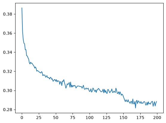

# put layers into eval mode for batchnorm
for layer in model.layers:
  layer.training = False

# evaluate the loss
@torch.no_grad() # this decorator disables gradient tracking inside pytorch
def split_loss(split):
  x,y = {
    'train': (Xtr, Ytr),
    'val': (Xdev, Ydev),
    'test': (Xte, Yte),
  }[split]

  logits = model(x)
  loss = F.cross_entropy(logits, y)
  print(split, loss.item())

split_loss('train')
split_loss('val')

train 1.9126217365264893
val 2.0188381671905518

# performance log:
# 3 character context:
train 2.0593066215515137
val 2.1068434715270996

8 character context:
train 1.9230281114578247
val 2.0320310592651367

current with wavenet and fix bug in batchnorm:
train 1.9126217365264893
val 2.0188381671905518

Implementation reflections¶

# sample from the model

for _ in range(20):

    out = []
    context = [0] * block_size #initialize with all ...

    while True:

        # forward pass the neural net
        logits = model(torch.tensor([context]))
        
        # # forward pass the neural net
        # emb = C[torch.tensor([context])]   # (1, block_size, n_embd)
        # x = emb.view(1, -1)                # (1, block_size*n_embd)
        
        # for layer in layers:
        #     x = layer(x)
        # logits = x
        probs = F.softmax(logits, dim=1)

        # sample from the distribution
        ix = torch.multinomial(probs, num_samples=1).item()

        # shift the context window and track the samples
        context = context[1:] + [ix]
        out.append(ix)
        # if we sample the special '.' token, break
        if ix == 0:
            break
        
    print(''.join(itos[i] for i in out)) # decode and print the generated word

kamon.
wlihanna.
franco.
jasler.
themi.
faynley.
matharynni.
blaylah.
hason.
celvi.
ajusleana.
kalypsa.
lanah.
marles.
conxann.
marna.
hozes.
shier.
mylen.
abreara.

# now, push our limits
# n_embd = 24, n_hidden = 128 to get 76000 parameters, training takes a lot longer, we can't bro, atleast not now, our laptop can't take it
# andrej got validation performance of 1.99
# but we're still in the dark about correct setting of the hyperparameters, learning rates, etc

# in our plot, we want to look at both training and validation loss, but currently, we're only looking at the training loss

# we implemented the architecture from the wavenet paper, but not forward pass circuit with complicated linear layer, residual connections, skip connections

# we want to preview, what we've done here relates to convolutional neural networks as used in wavenet paper
# use of convolutions is strictly for efficiency, it doesn't change the implemented model

for x, y in zip(Xtr[7:15], Ytr[7:15]):
    print(''.join(itos[ix.item()] for ix in x), '-->', itos[y.item()])

# our given name has 8 independent examples

........ --> h
.......h --> i
......hi --> l
.....hil --> t
....hilt --> o
...hilto --> n
..hilton --> .
........ --> j

# we're tricking 
print(Xtr[7].shape)
# model(Xtr[7]) gives error cuz its not a batch dimension
# so do Xtr[[7]] #a list of 7, thus its 1x7, and we can forward the model

torch.Size([8])

# forward a single example 
logits = model(Xtr[[7]])
logits.shape

torch.Size([1, 27])

# forward all 8 examples at the same time
logits = torch.zeros(8,27) #pre-allocating some memory
for i in range(8):
    logits[i] = model(Xtr[[7+i]]) #forward examples
logits.shape

torch.Size([8, 27])

# convolution is a "for loop"
# convolution allows us to forward Linear layers efficiently over space
# convolutions allow you to slide this model efficiently over the input sequence
# so this for Loop can be done not outside in Python but inside of kernels in Cuda
# and this for Loop gets hidden into the convolution

Open original image: wavenetdilutedlayers.png

# we've implemented a single black structure 
# we've implemented that and calculated a single output i.e. a single example 
# but what convolutions allow you to do is it allows you to take this black structure and kind of like slide it over the input sequence 
# and calculate all of these orange outputs at the same time 
# that corresponds to calculating all of these outputs at all the positions of the name with 8 examples at the same time

# why is this efficient?
# the for Loop is inside the Cuda kernels
# look at the variable reuse in the graph for some circles
# one node is the right child for some node and the left child for some other node elsewhere

# and we've pytorchified our code, kind of implemented torch.nn

# pytorch documentation is kinda incomplete, not so properly maintained, inconsistent, etc so finger crossed

# spend most of time making sure shapes of tensors are correct