Activations and normalization
Original study notes by Satish Bajagain, following Andrej Karpathy’s Zero to Hero. Comments, intermediate attempts and saved outputs are retained. Section titles are navigation additions.
Understanding activation statistics
# we want to move on to larger neural networks like recurrent neural networks and their variations like GRU, lstm, etc
# but before that we want to have a good understanding of activations in neural net during training
# and specially of the gradients that are flowing backwards, how they behave, and what they look like
# this is imp to understand the history of development of these architectures
# while RNN are expressive, they are a universal approximator and in principle can implement all algorithms
# we'll see that RNN are not very easily optimizable with the first order gradient based techniques that we use all the time
# to understand why RNN are not easily optimizable, we need to understand the activations and gradients and how they behave during training
# and we'll see that a lot of variants since RNN have tried to improve this situation
# starting code for this lecture is the same as before but minor tweaks that you'll understand easily, and with help of commentsimport torch
import torch.nn.functional as F
import matplotlib.pyplot as plt
%matplotlib inline# read all words
words = open("names.txt", "r").read().splitlines()
print(words[:8])
print(len(words))['emma', 'olivia', 'ava', 'isabella', 'sophia', 'charlotte', 'mia', 'amelia']
32033
# Build the vocabulary of characters and mappings to/from integers
chars = sorted(list(set(''.join(words))))
stoi = {s : i+1 for i, s in enumerate(chars)}
stoi['.'] = 0
itos = {i:s for s, i in stoi.items()}
vocab_size = len(itos)
print(itos)
print(vocab_size)
{1: 'a', 2: 'b', 3: 'c', 4: 'd', 5: 'e', 6: 'f', 7: 'g', 8: 'h', 9: 'i', 10: 'j', 11: 'k', 12: 'l', 13: 'm', 14: 'n', 15: 'o', 16: 'p', 17: 'q', 18: 'r', 19: 's', 20: 't', 21: 'u', 22: 'v', 23: 'w', 24: 'x', 25: 'y', 26: 'z', 0: '.'}
27
# build the dataset
# context length: how many characters do we take to predict the next one?
block_size = 3

def build_dataset(words):
    X, Y = [], []

    for w in words:
        context = [0] * block_size
        for ch in w + '.':
            ix = stoi[ch]
            X.append(context)
            Y.append(ix)
            context = context[1:] + [ix] #crop on left and append

    X = torch.tensor(X)
    Y = torch.tensor(Y)
    print(X.shape, Y.shape)
    return X, Y

import random
random.seed(42)
random.shuffle(words)
n1 = int(0.8 * len(words))
n2 = int(0.9 * len(words))

Xtr, Ytr = build_dataset(words[:n1]) #80%
Xdev, Ydev = build_dataset(words[n1:n2]) #10%
Xte, Yte = build_dataset(words[n2:]) #10%
torch.Size([182625, 3]) torch.Size([182625])
torch.Size([22655, 3]) torch.Size([22655])
torch.Size([22866, 3]) torch.Size([22866])
# MLP revisited
n_embd = 10 #dimensionality of the character embedding vectors
n_hidden = 200 #number of neurons in hidden layer of MLP

g = torch.Generator().manual_seed(2147483647) #use same seed for reproducibility
C = torch.randn((vocab_size, n_embd), generator = g)
W1 = torch.randn((n_embd * block_size, n_hidden), generator = g)
b1 = torch.randn(n_hidden, generator = g)
W2 = torch.randn((n_hidden, vocab_size), generator = g)
b2 = torch.randn(vocab_size, generator = g)

parameters = [C, W1, b1, W2, b2]
print(sum(p.nelement() for p in parameters))
for p in parameters:
    p.requires_grad = True
11897
# same optimization as previously done
max_steps = 200000
batch_size = 32
lossi = []

for i in range(max_steps):

    # minibatch construct
    ix = torch.randint(0, Xtr.shape[0], (batch_size, ), generator = g)
    Xb, Yb = Xtr[ix], Ytr[ix] #batch X, Y

    # forward pass
    emb = C[Xb] #embed the characters into vectors
    embcat = emb.view(emb.shape[0], -1) #concatenate the vectors
    hpreact = embcat @ W1 + b1 #hidden layer pre-activation
    h = torch.tanh(hpreact) #hidden layer
    logits = h @ W2 + b2 #output layer
    loss = F.cross_entropy(logits, Yb) #loss function

    # backward pass
    for p in parameters:
        p.grad = None
    loss.backward()

    # update
    lr = 0.1 if i < 100000 else 0.01 # step learning rate decay
    for p in parameters:
        p.data += -lr * p.grad

    # track stats
    if i % 1000 == 0: #print every once in a while
        print(f'{i:7d}/{max_steps:7d}: {loss.item():.4f}')
    lossi.append(loss.log10().item())
0/ 200000: 27.8817
1000/ 200000: 4.1661
2000/ 200000: 3.0921
3000/ 200000: 2.9381
4000/ 200000: 2.2535
5000/ 200000: 2.3730
6000/ 200000: 2.3974
7000/ 200000: 2.8007
8000/ 200000: 2.4276
9000/ 200000: 2.5784
10000/ 200000: 2.9571
11000/ 200000: 2.0548
12000/ 200000: 2.3778
13000/ 200000: 2.3974
14000/ 200000: 2.8170
15000/ 200000: 2.2712
16000/ 200000: 2.5917
17000/ 200000: 2.6650
18000/ 200000: 2.4507
19000/ 200000: 2.4330
20000/ 200000: 2.5722
21000/ 200000: 2.6016
22000/ 200000: 2.1298
23000/ 200000: 2.1793
24000/ 200000: 3.0445
25000/ 200000: 2.4252
26000/ 200000: 2.5052
27000/ 200000: 2.6437
28000/ 200000: 2.2556
29000/ 200000: 3.1923
30000/ 200000: 2.7646
31000/ 200000: 2.6741
32000/ 200000: 2.5378
33000/ 200000: 2.5036
34000/ 200000: 2.1476
35000/ 200000: 2.4872
36000/ 200000: 2.1147
37000/ 200000: 2.3196
38000/ 200000: 2.9486
39000/ 200000: 2.0292
40000/ 200000: 2.0305
41000/ 200000: 2.4910
42000/ 200000: 2.7686
43000/ 200000: 2.5346
44000/ 200000: 1.9142
45000/ 200000: 1.9151
46000/ 200000: 2.4361
47000/ 200000: 2.0344
48000/ 200000: 2.6735
49000/ 200000: 2.1647
50000/ 200000: 2.5794
51000/ 200000: 2.9069
52000/ 200000: 2.4059
53000/ 200000: 2.4307
54000/ 200000: 2.1391
55000/ 200000: 2.0361
56000/ 200000: 2.0808
57000/ 200000: 1.7228
58000/ 200000: 1.7367
59000/ 200000: 2.3184
60000/ 200000: 2.3242
61000/ 200000: 2.1974
62000/ 200000: 2.6087
63000/ 200000: 2.4233
64000/ 200000: 2.2013
65000/ 200000: 2.0786
66000/ 200000: 2.6614
67000/ 200000: 2.6344
68000/ 200000: 1.9336
69000/ 200000: 2.2588
70000/ 200000: 2.1174
71000/ 200000: 2.4858
72000/ 200000: 2.4512
73000/ 200000: 2.4317
74000/ 200000: 1.8438
75000/ 200000: 2.7360
76000/ 200000: 1.9129
77000/ 200000: 2.4255
78000/ 200000: 2.4489
79000/ 200000: 2.2000
80000/ 200000: 2.2993
81000/ 200000: 2.3183
82000/ 200000: 2.3165
83000/ 200000: 1.8720
84000/ 200000: 2.6831
85000/ 200000: 2.6265
86000/ 200000: 2.4700
87000/ 200000: 2.2398
88000/ 200000: 2.5135
89000/ 200000: 2.3752
90000/ 200000: 2.2481
91000/ 200000: 2.0835
92000/ 200000: 2.6384
93000/ 200000: 1.9178
94000/ 200000: 1.9773
95000/ 200000: 2.2083
96000/ 200000: 2.1389
97000/ 200000: 2.3097
98000/ 200000: 1.9052
99000/ 200000: 2.0819
100000/ 200000: 2.0146
101000/ 200000: 1.8770
102000/ 200000: 2.2421
103000/ 200000: 2.1059
104000/ 200000: 2.2212
105000/ 200000: 2.1796
106000/ 200000: 2.3958
107000/ 200000: 2.2501
108000/ 200000: 2.2253
109000/ 200000: 2.3500
110000/ 200000: 2.4534
111000/ 200000: 2.2884
112000/ 200000: 1.8768
113000/ 200000: 2.3609
114000/ 200000: 2.1293
115000/ 200000: 2.2429
116000/ 200000: 2.2294
117000/ 200000: 2.4280
118000/ 200000: 2.2524
119000/ 200000: 2.3136
120000/ 200000: 1.9164
121000/ 200000: 2.3675
122000/ 200000: 2.2222
123000/ 200000: 2.4959
124000/ 200000: 2.8668
125000/ 200000: 1.9559
126000/ 200000: 2.2162
127000/ 200000: 2.1895
128000/ 200000: 2.5736
129000/ 200000: 2.1753
130000/ 200000: 2.3719
131000/ 200000: 1.8927
132000/ 200000: 1.9425
133000/ 200000: 2.3153
134000/ 200000: 2.0467
135000/ 200000: 2.0507
136000/ 200000: 1.9243
137000/ 200000: 1.9577
138000/ 200000: 2.1316
139000/ 200000: 1.8914
140000/ 200000: 2.2377
141000/ 200000: 1.7482
142000/ 200000: 2.0938
143000/ 200000: 2.4556
144000/ 200000: 2.0439
145000/ 200000: 2.1131
146000/ 200000: 2.1402
147000/ 200000: 2.2063
148000/ 200000: 2.4627
149000/ 200000: 2.3908
150000/ 200000: 2.1441
151000/ 200000: 2.3513
152000/ 200000: 1.9725
153000/ 200000: 2.2721
154000/ 200000: 2.3124
155000/ 200000: 2.0890
156000/ 200000: 2.0114
157000/ 200000: 2.1071
158000/ 200000: 1.9900
159000/ 200000: 2.2106
160000/ 200000: 2.2661
161000/ 200000: 2.0200
162000/ 200000: 1.9794
163000/ 200000: 2.0711
164000/ 200000: 2.1216
165000/ 200000: 2.3295
166000/ 200000: 2.1930
167000/ 200000: 2.3925
168000/ 200000: 1.9545
169000/ 200000: 2.2910
170000/ 200000: 1.7855
171000/ 200000: 2.2078
172000/ 200000: 2.2121
173000/ 200000: 2.2136
174000/ 200000: 2.4515
175000/ 200000: 2.0452
176000/ 200000: 2.0188
177000/ 200000: 2.1216
178000/ 200000: 1.8341
179000/ 200000: 2.0375
180000/ 200000: 2.1126
181000/ 200000: 2.2063
182000/ 200000: 2.2261
183000/ 200000: 2.2427
184000/ 200000: 2.3953
185000/ 200000: 2.2676
186000/ 200000: 1.7918
187000/ 200000: 1.8241
188000/ 200000: 2.1250
189000/ 200000: 2.4299
190000/ 200000: 1.8004
191000/ 200000: 2.1577
192000/ 200000: 2.3515
193000/ 200000: 2.1037
194000/ 200000: 2.0033
195000/ 200000: 2.2219
196000/ 200000: 2.1530
197000/ 200000: 2.1457
198000/ 200000: 2.0172
199000/ 200000: 1.7894
# First thing we want to scrutinize(examine carefully) is the initialization
# we know that our network is very improperly configured at initialization
# at 0th iteration, loss = 27, and at 1000th iteration, it rapidly comes down at 4
# while training neural nets, we will always have a rough idea of what loss to expect at initialization which depends on loss function and problem setup
# what we'd like at initialization instead:
# so there's 27 characters that could come next right? at initialization we have no reason to believe any characters to be much more likely than others
# so initially, the probability distribution is a uniform distribution that assigns about equal probability to all 27 characters
# so for any char: prob is roughly 1/27.0
# and loss is the negative log probability which we can compute directly like this
1/27.0
torch.tensor(1/27.0).log()
-torch.tensor(1/27.0).log()tensor(3.2958)# so, initially our expected loss is 3.29, which is way lower than 27
# currently, at initialization: some characters are very confident and some are not confident due to randomly assigning probabilities initially
# so, the network is very confidently wrong which increases the loss by a lot# let's see a smaller 4-dimensional example of this issue
logits = torch.tensor([0.0, 0.0, 0.0, 0.0]) #suppose we have only 4 characters, and the logits that come out of neural net are very close to 0
probs = torch.softmax(logits, dim=0) #when we take a softmax of all 0's, we get probabilities that are diffused distribution
loss = -probs[2].log() #here, it doesn't matter if label is 0,1,2,3 cuz its a uniform distribution, they all sum to 1
probs, loss(tensor([0.2500, 0.2500, 0.2500, 0.2500]), tensor(1.3863))# lets experiment now and see how the loss is affected when values are diff w.r.t one another
logits = torch.tensor([0.0, 0.0, 5.0, 0.0]) #suppose we have only 4 characters, and the logits that come out of neural net are very close to 0
probs = torch.softmax(logits, dim=0) #when we take a softmax of all 0's, we get probabilities that are diffused distribution
loss = -probs[2].log() #here, it doesn't matter if label is 0,1,2,3 cuz its a uniform distribution, they all sum to 1
probs, loss
# in this case, the initialization of correct probability to the correct label is by chance, thus we are getting low loss
# look at index 2: 5 and we are setting loss for index 2 as well, now look at another example(tensor([0.0066, 0.0066, 0.9802, 0.0066]), tensor(0.0200))# this case is much more likely than randomly guessing correct weights, the loss is much higher
logits = torch.tensor([0.0, 5.0, 0.0, 0.0]) #suppose we have only 4 characters, and the logits that come out of neural net are very close to 0
probs = torch.softmax(logits, dim=0) #when we take a softmax of all 0's, we get probabilities that are diffused distribution
loss = -probs[2].log() #here, it doesn't matter if label is 0,1,2,3 cuz its a uniform distribution, they all sum to 1
probs, loss(tensor([0.0066, 0.9802, 0.0066, 0.0066]), tensor(5.0200))# for the below random initialization case, since the logits that come out are near 0, the loss is okay
# but suppose its x10, you'll see that because these are more extreme values, its unlikely to guess correctly, so you're confidently wrong and thus recording very high loss
# and if the logits are very extreme, you might get insane losses like infinity# logits = torch.tensor([0.0, 5.0, 0.0, 0.0]) #suppose we have only 4 characters, and the logits that come out of neural net are very close to 0
logits = torch.randn(4)
probs = torch.softmax(logits, dim=0) #when we take a softmax of all 0's, we get probabilities that are diffused distribution
loss = -probs[2].log() #here, it doesn't matter if label is 0,1,2,3 cuz its a uniform distribution, they all sum to 1
logits, probs, loss(tensor([-1.7050, 1.2582, 0.0039, 1.4227]),
tensor([0.0205, 0.3975, 0.1134, 0.4686]),
tensor(2.1769))# logits = torch.tensor([0.0, 5.0, 0.0, 0.0]) #suppose we have only 4 characters, and the logits that come out of neural net are very close to 0
logits = torch.randn(4) * 100
probs = torch.softmax(logits, dim=0) #when we take a softmax of all 0's, we get probabilities that are diffused distribution
loss = -probs[2].log() #here, it doesn't matter if label is 0,1,2,3 cuz its a uniform distribution, they all sum to 1
logits, probs, loss(tensor([ 35.4741, -104.2379, 9.5114, -151.8761]),
tensor([1.0000e+00, 0.0000e+00, 5.3033e-12, 0.0000e+00]),
tensor(25.9627))Initial predictions and confidence
SUMMARY: RANDOM INITIALIZATION LIKE THIS IS NOT GOOD, AND WE WANT THE LOGITS TO BE ROUGHLY ZERO WHEN THE NETWORK IS INITIALIZED
iNFACT, THE LOGITS DON'T HAVE TO BE 0, THEY JUST HAVE TO BE EQUAL
# SETTING ALL TO 1: OK CUZ OF NORMALIZATION INSIDE SOFTMAX LATER
logits = torch.tensor([1.0, 1.0, 1.0, 1.0]) #suppose we have only 4 characters, and the logits that come out of neural net are very close to 0
probs = torch.softmax(logits, dim=0) #when we take a softmax of all 0's, we get probabilities that are diffused distribution
loss = -probs[2].log() #here, it doesn't matter if label is 0,1,2,3 cuz its a uniform distribution, they all sum to 1
logits, probs, loss(tensor([1., 1., 1., 1.]),
tensor([0.2500, 0.2500, 0.2500, 0.2500]),
tensor(1.3863))# after optimization, our loss looks something like this:
plt.plot(lossi)[<matplotlib.lines.Line2D at 0x72ff55056a50>]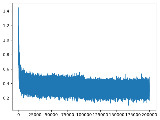
# this decorator disables gradient tracking
# when this decorator is used on top of a function
# torch assumes that whatever happens in this function never requires any gradients
# so it wont keep track of anything to keep track of gradients in anticipation of backward pass
# has the same effect as setting required_grad of all tensors here to false
# makes more efficient, cuz we let torch know that we wont call .backward() on any computation
# so torch doesnt have to maintain a graph under the hood
# you can also use a context manager with torch.no_grad

@torch.no_grad()
def split_loss(split):

    x, y = {
        'train': (Xtr, Ytr),
        'val': (Xdev, Ydev),
        'test': (Xte, Yte),
    }[split] #depending on train, val or test as input, index and get the correct split

    # forward pass of network: evaluate the loss and print it
    emb = C[x] # N x block_size x n_embd
    embcat = emb.view(emb.shape[0], -1) # concat into (N, block_size x n_embd) to allow matrix mul
    h = torch.tanh(embcat @ W1 + b1) # N x n_hidden
    logits = h @ W2 + b2 # N x vocab_size
    loss = F.cross_entropy(logits, y)
    print(split, loss.item())

split_loss('train')
split_loss('val')
train 2.1270017623901367
val 2.169905662536621
# sample from the model
g = torch.Generator().manual_seed(2147483647 + 10)
for _ in range(20):
out = []
context = [0] * block_size #initialize with all ...
while True:
# forward pass the neural net
emb = C[torch.tensor((context))] #(1, block_size, n_embd)
h = torch.tanh(emb.view(1, -1) @ W1 + b1)
logits = h @ W2 + b2
probs = F.softmax(logits, dim = 1)
# sample from the distribution
ix = torch.multinomial(probs, num_samples = 1, generator=g).item()
# shift the context window and track the samples
context = context[1:] + [ix]
out.append(ix)
# if we sample the special '.' then break
if ix == 0:
break
print(''.join(itos[i] for i in out)) #decode and print the generated wordcarlah.
amille.
khi.
mili.
taty.
skandeleja.
hutafaresara.
kaeli.
nellara.
chaiir.
kaleigh.
ham.
jorn.
quint.
salin.
alianni.
waztrogiearynix.
kael.
dura.
mer.
# the output is better, but still not amazing, and still not fully name like but way better than bigram model# so, where do things currently go wrong during initialization in our neural net?# same optimization as previously done
max_steps = 200000
batch_size = 32
lossi = []
for i in range(max_steps):
# minibatch construct
ix = torch.randint(0, Xtr.shape[0], (batch_size, ), generator = g)
Xb, Yb = Xtr[ix], Ytr[ix] #batch X, Y
# forward pass
emb = C[Xb] #embed the characters into vectors
embcat = emb.view(emb.shape[0], -1) #concatenate the vectors
hpreact = embcat @ W1 + b1 #hidden layer pre-activation
h = torch.tanh(hpreact) #hidden layer
logits = h @ W2 + b2 #output layer
loss = F.cross_entropy(logits, Yb) #loss function
# backward pass
for p in parameters:
p.grad = None
loss.backward()
# update
lr = 0.1 if i < 100000 else 0.01 # step learning rate decay
for p in parameters:
p.data += -lr * p.grad
# track stats
if i % 1000 == 0: #print every once in a while
print(f'{i:7d}/{max_steps:7d}: {loss.item():.4f}')
lossi.append(loss.log10().item())
break #break after the very first iteration itself 0/ 200000: 27.8817
# the loss is way too high, lets examine the logits randomly
# okay, so the logits take on extreme values, this creates fake confidence in incorrect answers thus increasing the loss
logits[5]
# so: these logits should be much much closer to zerotensor([-31.2260, 15.0341, 3.7797, -4.1423, 5.1893, 11.4668, 6.5744,
13.6292, -11.6972, -7.1791, 2.2053, 38.5218, -0.1899, -25.6748,
16.8003, 7.3650, 8.0879, -5.4867, -11.5406, -14.5259, 9.7959,
20.9665, -5.7736, -4.6396, 25.5794, 7.2416, 2.4288],
grad_fn=<SelectBackward0>)# how to make sure that logits coming out of neural net can be made much closer to zero?
# logits = h @ W2 + b2 #output layer
# we're initializing b2 as random values
# but now, since we want the logits to be roughly zero, we don't want to add any bias of random numbers to logits
# so at initialization, set b2 to 0, just multiply it by 0
# and if we want logits to be very small, we can multiply W2 to make it smaller, eg. multiply by 0.1 or 0.01 accordingly to scale down all elements
# MLP revisited
# ............................
# W2 = torch.randn((n_hidden, vocab_size), generator = g) * 0.1
# b2 = torch.randn(vocab_size, generator = g) * 0
# ........................# MLP revisited
n_embd = 10 #dimensionality of the character embedding vectors
n_hidden = 200 #number of neurons in hidden layer of MLP
g = torch.Generator().manual_seed(2147483647) #use same seed for reproducibility
C = torch.randn((vocab_size, n_embd), generator = g)
W1 = torch.randn((n_embd * block_size, n_hidden), generator = g)
b1 = torch.randn(n_hidden, generator = g)
W2 = torch.randn((n_hidden, vocab_size), generator = g) * 0.01 #scaling it down so it is near to 0 and logits will not be very extreme thus reducing loss at initialization itself
b2 = torch.randn(vocab_size, generator = g) * 0 #not adding anything at initialization to get low loss during first iteration itself
parameters = [C, W1, b1, W2, b2]
print(sum(p.nelement() for p in parameters))
for p in parameters:
p.requires_grad = True11897
# same optimization as previously done
max_steps = 200000
batch_size = 32
lossi = []
for i in range(max_steps):
# minibatch construct
ix = torch.randint(0, Xtr.shape[0], (batch_size, ), generator = g)
Xb, Yb = Xtr[ix], Ytr[ix] #batch X, Y
# forward pass
emb = C[Xb] #embed the characters into vectors
embcat = emb.view(emb.shape[0], -1) #concatenate the vectors
hpreact = embcat @ W1 + b1 #hidden layer pre-activation
h = torch.tanh(hpreact) #hidden layer
logits = h @ W2 + b2 #output layer
loss = F.cross_entropy(logits, Yb) #loss function
# backward pass
for p in parameters:
p.grad = None
loss.backward()
# update
lr = 0.1 if i < 100000 else 0.01 # step learning rate decay
for p in parameters:
p.data += -lr * p.grad
# track stats
if i % 1000 == 0: #print every once in a while
print(f'{i:7d}/{max_steps:7d}: {loss.item():.4f}')
lossi.append(loss.log10().item())
break #break after the very first iteration itself 0/ 200000: 3.3221
# WAAAAU: look that we are already much much closer to our expected loss at first iteration itself
# what we roughly want is 3.29 from -torch.tensor(1/27.0).log(). This is our reference
# currently when multiplying S2 by 0.01, we're getting a loss of 3.32
# but can we set W2 to multiply by 0 at initialization, it will ensure that we get exactly 3.29?
# but we don't want to set the weights of a neural net to exactly 0 at initialization because we are nervous of something
# so we set it to very small num instead of 0
# what is that something?# so we're not setting W2 to be exactly 0, but near 0: i.e. there is some entropy/randomness/uncertainity
# and this entropy is used for symmetry breaking# now, the logits are much closer to 0
logits[5]tensor([-0.3136, 0.1383, 0.0184, -0.0445, 0.0317, 0.1146, 0.0738, 0.1302,
-0.1349, -0.0651, 0.0348, 0.3965, -0.0048, -0.2584, 0.1568, 0.0671,
0.1079, -0.0677, -0.1155, -0.1388, 0.0844, 0.2292, -0.0689, -0.0466,
0.2477, 0.0804, 0.0268], grad_fn=<SelectBackward0>)# let's now run the optimization with this new initialization, and see what losses we record
# same optimization as previously done
max_steps = 200000
batch_size = 32
lossi = []
for i in range(max_steps):
# minibatch construct
ix = torch.randint(0, Xtr.shape[0], (batch_size, ), generator = g)
Xb, Yb = Xtr[ix], Ytr[ix] #batch X, Y
# forward pass
emb = C[Xb] #embed the characters into vectors
embcat = emb.view(emb.shape[0], -1) #concatenate the vectors
hpreact = embcat @ W1 + b1 #hidden layer pre-activation
h = torch.tanh(hpreact) #hidden layer
logits = h @ W2 + b2 #output layer
loss = F.cross_entropy(logits, Yb) #loss function
# backward pass
for p in parameters:
p.grad = None
loss.backward()
# update
lr = 0.1 if i < 100000 else 0.01 # step learning rate decay
for p in parameters:
p.data += -lr * p.grad
# track stats
if i % 10000 == 0: #print every once in a while
print(f'{i:7d}/{max_steps:7d}: {loss.item():.4f}')
lossi.append(loss.log10().item()) 0/ 200000: 3.3221
10000/ 200000: 2.1900
20000/ 200000: 2.4196
30000/ 200000: 2.6067
40000/ 200000: 2.0601
50000/ 200000: 2.4988
60000/ 200000: 2.3902
70000/ 200000: 2.1344
80000/ 200000: 2.3369
90000/ 200000: 2.1299
100000/ 200000: 1.8329
110000/ 200000: 2.2053
120000/ 200000: 1.8540
130000/ 200000: 2.4566
140000/ 200000: 2.1879
150000/ 200000: 2.1118
160000/ 200000: 1.8956
170000/ 200000: 1.8645
180000/ 200000: 2.0326
190000/ 200000: 1.8417
plt.plot(lossi)[<matplotlib.lines.Line2D at 0x72ff548e0ec0>]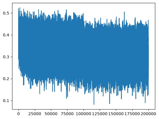
# now, we see that the plot of the loss doesn't have a hockey stick appearance
# cuz in that previous case, for the very first few iterations of the loss, the optimization is just squashing down the logits, then rearranging the logits
# but now, we took away the easy part of the loss function of rapid shrinking of loss
# now, the plot shows the hard gains of the neural net
# and the loss has improved quite a bit too@torch.no_grad()
def split_loss(split):
x, y = {
'train': (Xtr, Ytr),
'val': (Xdev, Ydev),
'test': (Xte, Yte),
}[split] #depending on train, val or test as input, index and get the correct split
# forward pass of network: evaluate the loss and print it
emb = C[x] # N x block_size x n_embd
embcat = emb.view(emb.shape[0], -1) # concat into (N, block_size x n_embd) to allow matrix mul
h = torch.tanh(embcat @ W1 + b1) # N x n_hidden
logits = h @ W2 + b2 # N x vocab_size
loss = F.cross_entropy(logits, y)
print(split, loss.item())
split_loss('train')
split_loss('val')train 2.069589138031006
val 2.1310746669769287
# previous loss log:
train 2.1270017623901367
val 2.169905662536621
# current loss log:
train 2.069589138031006
val 2.1310746669769287Hidden activations and saturation
# the reason why our result is improved is because: we're spending more cycles optimizing the neural net actually,
# instead of spending the first several thousands iterations squashing down the weights# Let's look at another problem now# MLP revisited
n_embd = 10 #dimensionality of the character embedding vectors
n_hidden = 200 #number of neurons in hidden layer of MLP
g = torch.Generator().manual_seed(2147483647) #use same seed for reproducibility
C = torch.randn((vocab_size, n_embd), generator = g)
W1 = torch.randn((n_embd * block_size, n_hidden), generator = g)
b1 = torch.randn(n_hidden, generator = g)
W2 = torch.randn((n_hidden, vocab_size), generator = g) * 0.01 #scaling it down so it is near to 0 and logits will not be very extreme thus reducing loss at initialization itself
b2 = torch.randn(vocab_size, generator = g) * 0 #not adding anything at initialization to get low loss during first iteration itself
parameters = [C, W1, b1, W2, b2]
print(sum(p.nelement() for p in parameters))
for p in parameters:
p.requires_grad = True11897
# same optimization as previously done
max_steps = 200000
batch_size = 32
lossi = []

for i in range(max_steps):

    # minibatch construct
    ix = torch.randint(0, Xtr.shape[0], (batch_size, ), generator = g)
    Xb, Yb = Xtr[ix], Ytr[ix] #batch X, Y

    # forward pass
    emb = C[Xb] #embed the characters into vectors
    embcat = emb.view(emb.shape[0], -1) #concatenate the vectors
    hpreact = embcat @ W1 + b1 #hidden layer pre-activation
    h = torch.tanh(hpreact) #hidden layer
    logits = h @ W2 + b2 #output layer
    loss = F.cross_entropy(logits, Yb) #loss function

    # backward pass
    for p in parameters:
        p.grad = None
    loss.backward()

    # update
    lr = 0.1 if i < 100000 else 0.01 # step learning rate decay
    for p in parameters:
        p.data += -lr * p.grad

    # track stats
    if i % 1000 == 0: #print every once in a while
        print(f'{i:7d}/{max_steps:7d}: {loss.item():.4f}')
    lossi.append(loss.log10().item())

    break #break after the very first iteration itself
0/ 200000: 3.3221
# though everything looks good on the level of loss, there's a deeper problem lurking inside this neural net and its initialization
# the logits are okay now, the problem now is with the values of h: the activations of the hidden states
# h = torch.tanh(hpreact)# LETS visualize the tensor h, notice that many of the elements are 1 or -1
print(h)
# recall that tanh is a squashing function, it takes arbitrary numbers and squashes them between the range of 1 and -1 smoothly
# lets look at the histogram of h to get a better idea of the distribution of the values inside this tensor
print(h.shape) #32 examples(our batch size) with 200 activations for each of the 32 examplestensor([[ 0.8100, -0.8997, -0.9993, ..., -0.9097, -1.0000, 1.0000],
[-1.0000, -0.9571, -0.7145, ..., 0.4898, 0.9090, 0.9937],
[ 0.9983, -0.3340, 1.0000, ..., 0.9443, 0.9905, 1.0000],
...,
[-1.0000, 0.9604, -0.1418, ..., -0.1266, 1.0000, 1.0000],
[-1.0000, -0.4385, -0.8882, ..., -0.3316, 0.9995, 1.0000],
[-1.0000, 0.9604, -0.1418, ..., -0.1266, 1.0000, 1.0000]],
grad_fn=<TanhBackward0>)
torch.Size([32, 200])
# we can stretch h out into a one large vector
print(h.view(-1).shape)
# then convert it into one large python list of floats
# h.view(-1).tolist()torch.Size([6400])
plt.hist(h.view(-1).tolist(), 50);
# semicolon to supress some output we don't want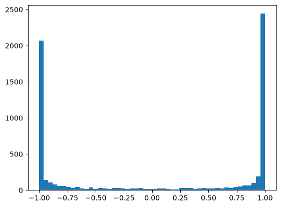
# from the histogram, we see that most of the values take on -1 and +1
# so our tanh is very very active, and to see why so, we can look at the preactivations
# hpreact = embcat @ W1 + b1 #hidden layer pre-activation
# h = torch.tanh(hpreact) #hidden layer
# logits = h @ W2 + b2 #output layer
# distribution of the preactivations is very broad: they take nums between -15 and 15, so in torch.tanh everything is being capped to be in range -1 to 1
# and lots of numbers take extreme value(-1, 1)
plt.hist(hpreact.view(-1).tolist(), 50);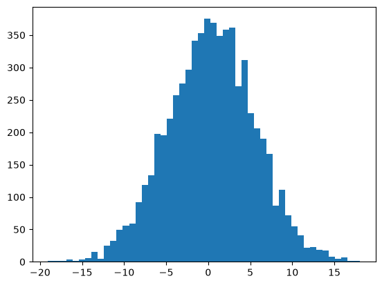
# if you're well versed in backpropagation, and have a sense of how gradients flow through this neural net, and looking at distributions of tanh activations
# you're sweating probably# Plot a histogram of tanh activations (using ~50 bins) to inspect how active the neurons are.
# Observation:
# - Most tanh outputs are either very close to -1 or +1.
# - This means many neurons are SATURATED.
# - Instead of producing a wide range of values, they are stuck at the extremes.
# To understand why, inspect the PRE-ACTIVATIONS (values before tanh).
# - Their distribution is very wide (e.g. roughly -5 to +15).
# - Large positive inputs become ~+1 after tanh.
# - Large negative inputs become ~-1 after tanh.
# - tanh squashes everything into the range [-1, 1], so large inputs get "clipped" to the ends.
# Why is this bad?
# - Saturated neurons create the VANISHING GRADIENT problem.
# - During backpropagation, gradients must pass through every tanh neuron.
# - If many neurons are saturated, gradients become tiny or even zero.
# Recall tanh implementation from micrograd:
# t = tanh(x)
# During backward pass:
# x.grad += (1 - t**2) * out.grad
# Here:
# - out.grad = gradient arriving from later layers.
# - (1 - t**2) = local derivative of tanh.
# - Chain rule multiplies them together.
# Case 1: t ≈ +1
# derivative = 1 - (1)^2 = 0
# x.grad = 0 * out.grad = 0
# Gradient completely dies.
# Case 2: t ≈ -1
# derivative = 1 - (-1)^2 = 0
# Same result: gradient becomes zero.
# Intuition:
# - At the flat tails of tanh, changing the input barely changes the output.
# - If the output barely changes, the loss barely changes.
# - Therefore there is almost nothing useful to learn.
# - The weights feeding this neuron receive almost no gradient updates.
# Case 3: t = 0
# derivative = 1 - 0^2 = 1
# x.grad = out.grad
# Gradient passes through unchanged.
# Important intuition:
# - The closer tanh output is to 0, the better gradients flow.
# - The closer tanh output is to ±1, the more gradients are squashed.
# - tanh can ONLY reduce gradient magnitude because:
# 0 <= (1 - t**2) <= 1
# - It never amplifies gradients; it either preserves or shrinks them.
# Goal during initialization:
# - Keep activations centered around 0 instead of saturating at ±1.
# - This allows gradients to flow through the network efficiently and makes learning much easier.# so our concern is, if all outputs h are in flat regions of -1 and 1, then the gradients flowing through the network will get destroyed at this layer during backpropplt.figure(figsize=(20,10))
plt.imshow(h.abs() > 0.99, cmap = 'gray', interpolation='nearest')
# we want to take absolute value of h and see how often it is in the flat line of tanh graph
# h.abs() > 0.99 is a boolean tensor: white if true and black if false
# graph shows 32 examples and 200 neurons: majority is white, they're in flat tail and the backward gradient would get destroyed
# we want to see more black instead of white<matplotlib.image.AxesImage at 0x72ff546dc550>
# we would be in deep trouble if for any one of the 200 neurons, the entire column was white: in that case, we have a dead neuron
# and it could be a tanh neuron where the initialization of the weights and biases could be such that no single example ever activates this tanh
# if all examples land in the tail, i.e. majority white, then this neuron will never learn: it is a dead neuron
# here thankfully, none of the neurons are completely white, and some examples do activate all neurons
# some gradients will flow through the neuron and the neuron will learn, the neuron will do something
# this is true for other non-linearities like sigmoid and relu
# you can easily get a dead relu neuron : its weights and biases will never get a gradient, can happen during initialization and optimization
# eg. if learning rate is too high, sometimes a neuron gets too much gradient and they get knocked out of data manifold,
# then no example ever activates that neuron forever, and its like a permanent brain damage in the mind of the network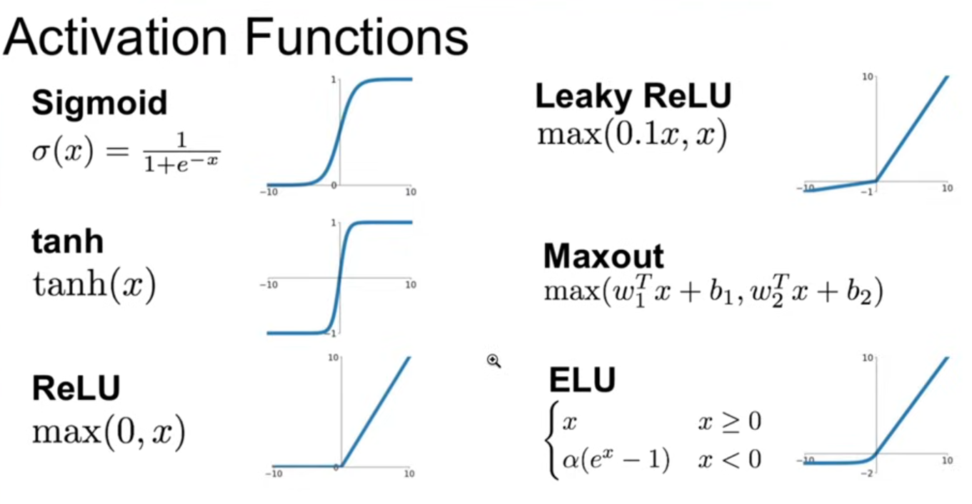
# other non-linearities like leaky relu don't suffer from this issue as much cuz it doesn't have flat tails
# and you'll almost always get gradients
# elu might suffer from this issue cuz it has flat parts# the h preactivation is too large and creating distributions too saturated on both sides of tanh
# and that's not good, cuz there's less training for these neurons and they update less frequently
# hpreact comes from C which is uniform gaussian(normal distribution) and W1 and b1
# hpreact is too far away from 0 which causes the issue, so like logits, we want hpreact to be closer to zero# we can multiply b1 by small num, we want to get a little bit of variation/entropy in the original initialization of tanh neurons
# and in practice, it helps optimization a little bit
# and also multiply W1 by small num like 0.1 too# MLP revisited
n_embd = 10 #dimensionality of the character embedding vectors
n_hidden = 200 #number of neurons in hidden layer of MLP
g = torch.Generator().manual_seed(2147483647) #use same seed for reproducibility
C = torch.randn((vocab_size, n_embd), generator = g)
W1 = torch.randn((n_embd * block_size, n_hidden), generator = g) * 0.1 #added this
b1 = torch.randn(n_hidden, generator = g) * 0.01 #added this
W2 = torch.randn((n_hidden, vocab_size), generator = g) * 0.01 #scaling it down so it is near to 0 and logits will not be very extreme thus reducing loss at initialization itself
b2 = torch.randn(vocab_size, generator = g) * 0 #not adding anything at initialization to get low loss during first iteration itself
parameters = [C, W1, b1, W2, b2]
print(sum(p.nelement() for p in parameters))
for p in parameters:
p.requires_grad = True11897
# rerun the first batch only# same optimization as previously done
max_steps = 200000
batch_size = 32
lossi = []
for i in range(max_steps):
# minibatch construct
ix = torch.randint(0, Xtr.shape[0], (batch_size, ), generator = g)
Xb, Yb = Xtr[ix], Ytr[ix] #batch X, Y
# forward pass
emb = C[Xb] #embed the characters into vectors
embcat = emb.view(emb.shape[0], -1) #concatenate the vectors
hpreact = embcat @ W1 + b1 #hidden layer pre-activation
h = torch.tanh(hpreact) #hidden layer
logits = h @ W2 + b2 #output layer
loss = F.cross_entropy(logits, Yb) #loss function
# backward pass
for p in parameters:
p.grad = None
loss.backward()
# update
lr = 0.1 if i < 100000 else 0.01 # step learning rate decay
for p in parameters:
p.data += -lr * p.grad
# track stats
if i % 1000 == 0: #print every once in a while
print(f'{i:7d}/{max_steps:7d}: {loss.item():.4f}')
lossi.append(loss.log10().item())
break #break after the very first iteration itself 0/ 200000: 3.3069
plt.hist(h.view(-1).tolist(), 50);
# semicolon to supress some output we don't want
# wow, look at the difference in output: it was more towards 1 and -1 previously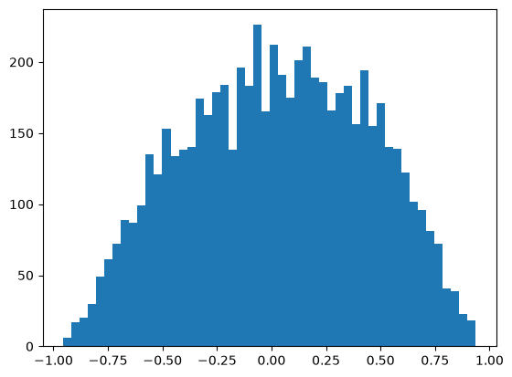
plt.hist(hpreact.view(-1).tolist(), 50);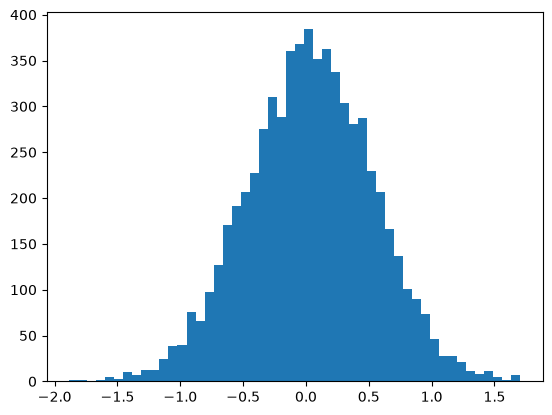
# now the preactivations are from -1.5 to 1.5 instead of -15 to 15plt.figure(figsize=(20,10))
plt.imshow(h.abs() > 0.99, cmap = 'gray', interpolation='nearest')<matplotlib.image.AxesImage at 0x72ff54309bd0>
# currently, there are no neurons that saturated over 0.99
# slightly adjust, now multiplying W1 by 0.2 instead to get even distribution, also include some saturated neurons# MLP revisited
n_embd = 10 #dimensionality of the character embedding vectors
n_hidden = 200 #number of neurons in hidden layer of MLP
g = torch.Generator().manual_seed(2147483647) #use same seed for reproducibility
C = torch.randn((vocab_size, n_embd), generator = g)
W1 = torch.randn((n_embd * block_size, n_hidden), generator = g) * 0.2 #changed this from 0.1 to 0.2
b1 = torch.randn(n_hidden, generator = g) * 0.01 #added this
W2 = torch.randn((n_hidden, vocab_size), generator = g) * 0.01 #scaling it down so it is near to 0 and logits will not be very extreme thus reducing loss at initialization itself
b2 = torch.randn(vocab_size, generator = g) * 0 #not adding anything at initialization to get low loss during first iteration itself
parameters = [C, W1, b1, W2, b2]
print(sum(p.nelement() for p in parameters))
for p in parameters:
p.requires_grad = True11897
# same optimization as previously done
max_steps = 200000
batch_size = 32
lossi = []

for i in range(max_steps):

    # minibatch construct
    ix = torch.randint(0, Xtr.shape[0], (batch_size, ), generator = g)
    Xb, Yb = Xtr[ix], Ytr[ix] #batch X, Y

    # forward pass
    emb = C[Xb] #embed the characters into vectors
    embcat = emb.view(emb.shape[0], -1) #concatenate the vectors
    hpreact = embcat @ W1 + b1 #hidden layer pre-activation
    h = torch.tanh(hpreact) #hidden layer
    logits = h @ W2 + b2 #output layer
    loss = F.cross_entropy(logits, Yb) #loss function

    # backward pass
    for p in parameters:
        p.grad = None
    loss.backward()

    # update
    lr = 0.1 if i < 100000 else 0.01 # step learning rate decay
    for p in parameters:
        p.data += -lr * p.grad

    # track stats
    if i % 1000 == 0: #print every once in a while
        print(f'{i:7d}/{max_steps:7d}: {loss.item():.4f}')
    lossi.append(loss.log10().item())

    break #break after the very first iteration itself
0/ 200000: 3.3135
plt.hist(h.view(-1).tolist(), 50);
# semicolon to supress some output we don't want
# now, this is a nice distribution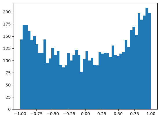
plt.hist(hpreact.view(-1).tolist(), 50);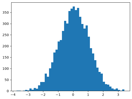
plt.figure(figsize=(20,10))
plt.imshow(h.abs() > 0.99, cmap = 'gray', interpolation='nearest')<matplotlib.image.AxesImage at 0x72ff4d7e0f50>
# now, run the full optimization without the break at first iteration after resetting the parameters ofcourse# same optimization as previously done
max_steps = 200000
batch_size = 32
lossi = []
for i in range(max_steps):
# minibatch construct
ix = torch.randint(0, Xtr.shape[0], (batch_size, ), generator = g)
Xb, Yb = Xtr[ix], Ytr[ix] #batch X, Y
# forward pass
emb = C[Xb] #embed the characters into vectors
embcat = emb.view(emb.shape[0], -1) #concatenate the vectors
hpreact = embcat @ W1 + b1 #hidden layer pre-activation
h = torch.tanh(hpreact) #hidden layer
logits = h @ W2 + b2 #output layer
loss = F.cross_entropy(logits, Yb) #loss function
# backward pass
for p in parameters:
p.grad = None
loss.backward()
# update
lr = 0.1 if i < 100000 else 0.01 # step learning rate decay
for p in parameters:
p.data += -lr * p.grad
# track stats
if i % 10000 == 0: #print every once in a while
print(f'{i:7d}/{max_steps:7d}: {loss.item():.4f}')
lossi.append(loss.log10().item()) 0/ 200000: 3.3135
10000/ 200000: 2.1648
20000/ 200000: 2.3061
30000/ 200000: 2.4541
40000/ 200000: 1.9787
50000/ 200000: 2.2930
60000/ 200000: 2.4232
70000/ 200000: 2.0680
80000/ 200000: 2.3095
90000/ 200000: 2.1207
100000/ 200000: 1.8269
110000/ 200000: 2.2045
120000/ 200000: 1.9797
130000/ 200000: 2.3946
140000/ 200000: 2.1000
150000/ 200000: 2.1948
160000/ 200000: 1.8619
170000/ 200000: 1.7809
180000/ 200000: 1.9673
190000/ 200000: 1.8295
@torch.no_grad()
def split_loss(split):

    x, y = {
        'train': (Xtr, Ytr),
        'val': (Xdev, Ydev),
        'test': (Xte, Yte),
    }[split] #depending on train, val or test as input, index and get the correct split

    # forward pass of network: evaluate the loss and print it
    emb = C[x] # N x block_size x n_embd
    embcat = emb.view(emb.shape[0], -1) # concat into (N, block_size x n_embd) to allow matrix mul
    h = torch.tanh(embcat @ W1 + b1) # N x n_hidden
    logits = h @ W2 + b2 # N x vocab_size
    loss = F.cross_entropy(logits, y)
    print(split, loss.item())

split_loss('train')
split_loss('val')
train 2.0355966091156006
val 2.1026785373687744
# previous loss log:
train 2.1270017623901367
val 2.169905662536621
# previous loss log:
train 2.069589138031006
val 2.1310746669769287
# current loss log(better):
train 2.0355966091156006
val 2.1026785373687744Scaling initialization
# why are our results better?
# our initialization is better, we're spending more time doing productive training instead of previous one where most gradients were set to 0
# this illustrates impact of initialization on performance by being aware of the internals of the neural nets and their activations and their gradients
# we're working with a very small network: single layer MLP, so since the network is so shallow, the optimization problem is very easy
# so though our initialization is terrible, the network eventually learned
# but this case doesn't occur in general, once we start working with deeper networks that have eg. 50 layers
# and if your initialization is bad, your network might not even train at all
# more complex the network, less forgiving it is to errors# now, how did we come up with the magic numbers: 0.1, 0.2, 0.01 earlier to modify the initialization of weights and biases
# what to do incase of a large neural net with lots and lots of layers
# there are some principled ways to set those numbersx = torch.randn(1000, 10) # 1000 x 10 tensor: 1000 examples that are 10-dimensional each
w = torch.randn(10, 200) # 10 x 200 tensor #weight layer also initialized using Gaussian/Normal/Bell shaped distribution, #200 neurons in the hidden layer look at 10 input each
y = x @ w #1000 x 200 tensor #get the preactivations of the neurons #for now, forget bias and non-linearity
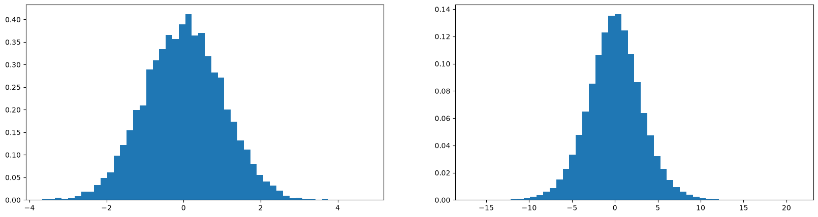
print(x.mean(), x.std())
print(y.mean(), y.std())
plt.figure(figsize=(20, 5))
plt.subplot(121)
plt.hist(x.view(-1).tolist(), 50, density=True);
plt.subplot(122)
plt.hist(y.view(-1).tolist(), 50, density=True);
# initially mean/s.d. of x and w = 0/1. we are curious about how the nature of y will be
# so the mean and s.d. of the gaussian/normal distribution
# s.d: just the spread of the gaussian/normal distribution
# we notice that y.mean stays the same: about 0 cuz its a symmetric operation, but the s.d. has expanded to 3 from 1
# but we don't want that, we want the neural net to have mostly similar activations, roughly unit Gaussian throughout the neural net
# so, now the qn is: how do we scale/multiply the W with to preserve the distribution to remain gaussian, i.e. to ensure that s.d. of y will also be 1 later after matrix multiplicationtensor(0.0035) tensor(1.0100)
tensor(-0.0125) tensor(3.1737)
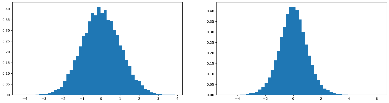
# now, the correct answer is that we are supposed to divide by the square root of the fan_in
# fan_in: the no of input elements in W, in above case: 10, so divide by square root of 10x = torch.randn(1000, 10) # 1000 x 10 tensor: 1000 examples that are 10-dimensional each
w = torch.randn(10, 200) / (10 ** 0.5) #200 neurons in the hidden layer look at 10 input each
y = x @ w #1000 x 200 tensor #get the preactivations of the neurons #for now, forget bias and non-linearity
print(x.mean(), x.std())
print(y.mean(), y.std())
plt.figure(figsize=(20, 5))
plt.subplot(121)
plt.hist(x.view(-1).tolist(), 50, density=True);
plt.subplot(122)
plt.hist(y.view(-1).tolist(), 50, density=True);tensor(0.0047) tensor(0.9983)
tensor(4.0914e-05) tensor(1.0165)
# a number of papers have looked into best initialized neural networks, and in case of MLP, we can have deep networks with non-linearities in between
# we want to make sure that the activations are well-behaved and they don't expand to infinity or shrink all the way to 0
# so how do we initialize the weights so the activations take on reasonable values throughout the network?
# a paper Kaiming He that has studied this in detail and is often cited: Delving Deep into Rectifiers# in the paper, they study the relu and prelu nonlinearity, but the analysis is very similar
# relu is a squashing function where all the negative numbers are simply clamped to zero, and positive numbers are pass through
# and because you're throwing away half the distribution, from their analysis of forward forward activations in the neural net
# you have to compensate for that with a gain
# i.e. they have to initialize their weights with a zero-mean Gaussian whose standard deviation is square root of 2 over fan_in
# "from paper
# This leads to a zero-mean Gaussian distribution whose standard deviation (std) is √2/nl.
# This is our way of initialization.
# "
# they have to add a factor of 2 cuz of relu which discards half of the distribution
# this kind of initialization is also implemented in pytorch# look at the torch.nn.init.kaiming_normal_(tensor, a=0, mode='fan_in', nonlinearity='leaky_relu', generator=None) part
# currently, this is the most common way of initializing neural networks
# it takes a few arguments
# 1. mode: would you like to normalize the activations or normalize the gradients to be always gaussian with 0 mean and 1 s.d.?
# it doesn't matter to much, so leave it at fan_in
# 2. passing the non_linearity that you're using, cuz depending on non-linearity, we need to calculate a slightly different gain
# if we pass no non-linearity, gain will be 1 as in above case, in case of relu, gain is square root of 2 which you can see in the top, because it was so in the paper# incase of tanh, advised gain is 5/3
# why do we need a gain on top of the initialization?
# its cus tanh, relu are contractive transformation: the output distribution from the matrix multiplication will be squashed in some way
# relu squashes by clamping everything below 0 to 0
# tanh will take the tails and then squeeze them in. so to fight the squeeze, we need to boost the weights a little bit so that we renormalize everything back to unit(1) s.d
# that's why there's a little bit of gain# about 7-9 years ago, everything was very fragile, the gradients, activations, histograms, scrutinizing non-linearities, etc specially if the neural net was deep
# modern innovations have made everything more stable and well behaved
# so its become less important to initialize these networks exactly right
# some modern innovations: 1. residual connections,
# 2. use of number of normalization layers eg. batch normalization, layer normalization, group normalization
# 3. much better optimizers, not just stochastic gradient descent, but complex ones like RMS PROP and adam
# due to these innovations, it is less imp to precisely calibrate the initialization of the neural net# in practice, what do we do then?
# just normalize the weights by the square root of the fan_in
# to be exactly accurate, std=(gain/fan_mode)**0.5
# https://docs.pytorch.org/docs/2.13/nn.init.html#torch-nn-init# to set the s.d. of our weights, do the following:# create 10k numbers and look at the std
# its the spread of the Gaussian/Normal distribution with mean 0 and s.d. 1
torch.randn(1000).std()tensor(1.0118)# multiply it by 0.2 to get s.d of 0.2
(torch.randn(1000) * 0.2).std()
# what we're trying to show is the num we multiply with there ends up being the s.d. of the gaussiantensor(0.1980)# W1 = torch.randn((n_embd * block_size, n_hidden), generator = g) * 0.2
# this ensured a s.d. of 0.2 gaussian when we sample our W1
# but we want to set the s.d. to square root of gain/fan_in# from documentation: gain for tanh : 5/3# gain / (fan_in)**(-n)
# gain divided by square root of fan_in
# the fan_in for W1 was n_embd * block_size which is 30. yes n_embd=10 but we had 3 of them and concatenated them so we should have used 30 instead of 10 in mini example of x, w and y = x @ w
(5/3) / (30 ** 0.5)
# this number is what we want our standard deviation to be0.3042903097250923# W1 = torch.randn((n_embd * block_size, n_hidden), generator = g) * 0.2
# we're going to replace that 0.2 with something better now
# instead of 0.2, use:
# (5/3) / ((n_embd * block_size) ** 0.5)
# So,
# W1 = torch.randn((n_embd * block_size, n_hidden), generator = g) * (5/3) / ((n_embd * block_size) ** 0.5)
# so, this is how we want to initialize our neural net's weights for tanh non-linearity# so that's what we'll do, and see what we get(5/3) / ((n_embd * block_size) ** 0.5)0.3042903097250923# MLP revisited
n_embd = 10 #dimensionality of the character embedding vectors
n_hidden = 200 #number of neurons in hidden layer of MLP
g = torch.Generator().manual_seed(2147483647) #use same seed for reproducibility
C = torch.randn((vocab_size, n_embd), generator = g)
W1 = torch.randn((n_embd * block_size, n_hidden), generator = g) * (5/3) / ((n_embd * block_size) ** 0.5)
b1 = torch.randn(n_hidden, generator = g) * 0.01 #added this
W2 = torch.randn((n_hidden, vocab_size), generator = g) * 0.01 #scaling it down so it is near to 0 and logits will not be very extreme thus reducing loss at initialization itself
b2 = torch.randn(vocab_size, generator = g) * 0 #not adding anything at initialization to get low loss during first iteration itself
parameters = [C, W1, b1, W2, b2]
print(sum(p.nelement() for p in parameters))
for p in parameters:
p.requires_grad = True11897
# same optimization as previously done
max_steps = 200000
batch_size = 32
lossi = []

for i in range(max_steps):

    # minibatch construct
    ix = torch.randint(0, Xtr.shape[0], (batch_size, ), generator = g)
    Xb, Yb = Xtr[ix], Ytr[ix] #batch X, Y

    # forward pass
    emb = C[Xb] #embed the characters into vectors
    embcat = emb.view(emb.shape[0], -1) #concatenate the vectors
    hpreact = embcat @ W1 + b1 #hidden layer pre-activation
    h = torch.tanh(hpreact) #hidden layer
    logits = h @ W2 + b2 #output layer
    loss = F.cross_entropy(logits, Yb) #loss function

    # backward pass
    for p in parameters:
        p.grad = None
    loss.backward()

    # update
    lr = 0.1 if i < 100000 else 0.01 # step learning rate decay
    for p in parameters:
        p.data += -lr * p.grad

    # track stats
    if i % 10000 == 0: #print every once in a while
        print(f'{i:7d}/{max_steps:7d}: {loss.item():.4f}')
    lossi.append(loss.log10().item())
0/ 200000: 3.3179
10000/ 200000: 2.1910
20000/ 200000: 2.3270
30000/ 200000: 2.5396
40000/ 200000: 1.9468
50000/ 200000: 2.3331
60000/ 200000: 2.3852
70000/ 200000: 2.1173
80000/ 200000: 2.3159
90000/ 200000: 2.2010
100000/ 200000: 1.8591
110000/ 200000: 2.0881
120000/ 200000: 1.9389
130000/ 200000: 2.3913
140000/ 200000: 2.0949
150000/ 200000: 2.1458
160000/ 200000: 1.7824
170000/ 200000: 1.7249
180000/ 200000: 1.9752
190000/ 200000: 1.8614
plt.plot(lossi)[<matplotlib.lines.Line2D at 0x72ff5616f0e0>]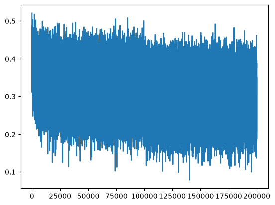
@torch.no_grad()
def split_loss(split):

    x, y = {
        'train': (Xtr, Ytr),
        'val': (Xdev, Ydev),
        'test': (Xte, Yte),
    }[split] #depending on train, val or test as input, index and get the correct split

    # forward pass of network: evaluate the loss and print it
    emb = C[x] # N x block_size x n_embd
    embcat = emb.view(emb.shape[0], -1) # concat into (N, block_size x n_embd) to allow matrix mul
    h = torch.tanh(embcat @ W1 + b1) # N x n_hidden
    logits = h @ W2 + b2 # N x vocab_size
    loss = F.cross_entropy(logits, y)
    print(split, loss.item())

split_loss('train')
split_loss('val')
train 2.0376641750335693
val 2.106989622116089
# previous loss log:
train 2.1270017623901367
val 2.169905662536621
# previous loss log:
train 2.069589138031006
val 2.1310746669769287
# previous loss log
train 2.0355966091156006
val 2.1026785373687744
# current loss log
train 2.0376641750335693
val 2.106989622116089Batch normalization
# so after initializing W1 like that, we still got roughly the same loss
# but the big deal is that we didn't have to use magic numbers we got looking from histograms and guess and checking
# we now use something semi-principled, and will scale us to much bigger networks
# the precise setup of the magic numbers during initializations is not so imp today due to some modern innovations
# one of those modern innovations is batch normalization# we were talking about how hpreact shouldn't be too small, then the tanh isn't doing anything
# but we also don't want it to be too large, then the tanh becomes saturated and gradients don't flow
# what we want is for hpreact to be roughly Gaussian: so mean: 0 and S.D.:1 at initialization# Insight from batch normalization paper:
# just take the hidden states and normalize them to be Gaussian
# just normalize the preactivation before it goes into the tanh brohpreact.shapetorch.Size([32, 200])# calculate mean across the 0th dimension (vertically down) and keepdims = True to make it easily broadcastable
hpreact.mean(0, keepdim=True)
hpreact.std(0, keepdim=True)tensor([[1.9613, 1.3486, 2.6169, 2.9698, 2.7784, 2.1968, 2.1737, 3.2098, 1.8199,
1.9680, 1.8995, 1.9896, 1.0719, 2.4876, 1.9648, 1.7460, 2.8172, 2.7818,
2.6821, 2.4640, 2.6209, 3.3153, 1.6177, 2.3900, 2.4985, 1.7149, 2.0246,
2.5168, 2.8657, 2.4524, 1.6224, 1.8967, 2.7732, 1.6037, 1.5137, 2.2101,
2.4012, 2.3304, 2.0241, 1.8732, 1.4424, 2.1492, 1.6517, 1.5745, 1.8599,
1.9858, 1.9352, 2.8817, 1.7111, 2.4724, 2.0803, 2.0884, 1.9877, 2.0851,
1.7538, 2.4325, 1.8240, 2.4118, 2.6271, 1.5493, 1.7387, 2.2251, 1.7173,
1.3836, 2.9623, 1.6185, 1.7514, 2.0846, 2.2292, 2.5178, 2.4438, 1.4803,
1.5512, 2.4341, 1.5833, 1.7891, 2.3643, 2.0278, 1.3426, 2.3906, 1.8960,
2.4052, 1.6073, 2.6124, 2.5638, 2.3395, 1.9467, 2.4481, 2.1223, 2.2247,
2.2783, 2.2455, 1.9989, 2.1343, 2.4529, 1.8233, 2.5712, 1.5163, 2.1924,
2.2142, 2.3564, 2.3831, 2.9241, 2.2520, 1.9678, 1.5307, 2.4070, 1.6361,
2.2437, 1.4952, 2.4418, 2.5749, 1.8294, 2.2800, 2.1689, 2.5579, 1.6360,
2.2833, 2.2701, 2.9364, 1.6848, 2.6299, 1.6085, 2.5661, 2.6057, 1.8512,
1.8815, 1.6132, 1.9918, 1.3530, 2.6038, 2.5717, 1.9360, 2.5749, 1.6645,
1.8305, 1.9283, 2.4305, 1.7599, 1.9086, 2.3116, 2.5427, 1.9926, 1.7846,
2.6498, 2.1044, 1.8586, 1.4043, 1.9260, 1.5291, 2.7683, 2.6458, 2.0966,
2.1427, 1.5872, 1.9787, 2.3137, 2.0506, 1.8957, 2.4453, 1.9769, 1.6061,
2.1647, 2.6291, 2.0988, 1.2304, 3.1327, 1.9531, 2.4582, 1.9261, 2.1413,
2.2315, 2.2603, 1.4084, 3.1167, 2.3562, 2.9757, 2.1950, 2.9440, 1.7912,
1.2578, 3.0028, 2.5685, 1.4476, 2.6790, 2.2613, 2.6849, 1.4139, 2.0182,
2.3849, 1.7070, 1.8136, 1.6201, 1.5524, 1.8777, 1.6591, 2.2013, 1.4714,
1.7916, 1.7215]], grad_fn=<StdBackward0>)hpreact.mean(0, keepdim=True).shapetorch.Size([1, 200])hpreact.std(0, keepdim=True).shapetorch.Size([1, 200])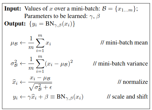
# mean: average of neurons activation
# s.d: distance of every value away from the mean, its just the spread, that squared and averaged gives variance, sq root of variance gives s.d.
# then normalize/standardize the x values by subtracting the mean by them and dividing by s.d.
# hpreact = (hpreact - hpreact.mean(0, keepdim=True)) / hpreact.std(0, keepdim = True)
# so every single neuron and its firing rate will be exactly Gaussian on the 32 examples i.e. on this batch, so its called batch normalization
# mean, sd are just mathematical formulas and are perfectly differentiable
# the epsilon is a small fixed number and its just preventing a division by 0 in the case that the variance over our batch is exactly 0, so things will be more well behaved
# though we haven't done it below cuz its unlikely to happen in a batch, feel free to add epsilon here,
# hpreact = bngain * (hpreact - bnmean_running) / (bnstd_running + epsilon) + bnbias
# we can just train this, but we won't achieve a very good result
# cuz we want it to be roughly Gaussian but only at initialization: we don't want to force hpreact to always be Gaussian
# we want to make it so that neural net can make it more diffused/sharp, make some tanh neurons more/less trigger happy# so in the paper, look at 4th formula, we take the normalized inputs, then additionally scaling them by some gain and offsetting them by some bias to get final output
# so we will allow a batch normalization gain to be initialized at 1's
# bngain = torch.ones((1, n_hidden))
# bnbias = torch.zeros((1, n_hidden))
# then
# our batch normalization layer:
# hpreact = bngain * (hpreact - hpreact.mean(0, keepdim=True)) / hpreact.std(0, keepdim = True) + bnbias
# since at initialization bngain is initialized to 1 and bnbias to 0, each neurons firing values in this batch will be unit Gaussian no matter the distribution of hpreact coming in
# so we got what we want at initialization
# don't forget to include these parameters in the list of parameters as they will be trained by the backpropagation
# during optimization, we'll be able to backpropagate into bngain and bnbias and change them so that the network has full ability to do whatever it wants internally(not forcing Gaussian distribution)# MLP revisited
n_embd = 10 #dimensionality of the character embedding vectors
n_hidden = 200 #number of neurons in hidden layer of MLP
g = torch.Generator().manual_seed(2147483647) #use same seed for reproducibility
C = torch.randn((vocab_size, n_embd), generator = g)
W1 = torch.randn((n_embd * block_size, n_hidden), generator = g) * (5/3) / ((n_embd * block_size) ** 0.5)
b1 = torch.randn(n_hidden, generator = g) * 0.01 #added this
W2 = torch.randn((n_hidden, vocab_size), generator = g) * 0.01 #scaling it down so it is near to 0 and logits will not be very extreme thus reducing loss at initialization itself
b2 = torch.randn(vocab_size, generator = g) * 0 #not adding anything at initialization to get low loss during first iteration itself
bngain = torch.ones((1, n_hidden))
bnbias = torch.zeros((1, n_hidden))
parameters = [C, W1, b1, W2, b2, bngain, bnbias]
print(sum(p.nelement() for p in parameters))
for p in parameters:
p.requires_grad = True12297
# same optimization as previously done
max_steps = 200000
batch_size = 32
lossi = []

for i in range(max_steps):

    # minibatch construct
    ix = torch.randint(0, Xtr.shape[0], (batch_size, ), generator = g)
    Xb, Yb = Xtr[ix], Ytr[ix] #batch X, Y

    # forward pass
    emb = C[Xb] #embed the characters into vectors
    embcat = emb.view(emb.shape[0], -1) #concatenate the vectors
    hpreact = embcat @ W1 + b1 #hidden layer pre-activation

    hpreact = bngain * (hpreact - hpreact.mean(0, keepdim=True)) / hpreact.std(0, keepdim=True) + bnbias

    h = torch.tanh(hpreact) #hidden layer
    logits = h @ W2 + b2 #output layer
    loss = F.cross_entropy(logits, Yb) #loss function

    # backward pass
    for p in parameters:
        p.grad = None
    loss.backward()

    # update
    lr = 0.1 if i < 100000 else 0.01 # step learning rate decay
    for p in parameters:
        p.data += -lr * p.grad

    # track stats
    if i % 10000 == 0: #print every once in a while
        print(f'{i:7d}/{max_steps:7d}: {loss.item():.4f}')
    lossi.append(loss.log10().item())
0/ 200000: 3.3147
10000/ 200000: 2.1984
20000/ 200000: 2.3375
30000/ 200000: 2.4359
40000/ 200000: 2.0119
50000/ 200000: 2.2595
60000/ 200000: 2.4775
70000/ 200000: 2.1020
80000/ 200000: 2.2788
90000/ 200000: 2.1862
100000/ 200000: 1.9474
110000/ 200000: 2.3010
120000/ 200000: 1.9837
130000/ 200000: 2.4523
140000/ 200000: 2.3839
150000/ 200000: 2.1987
160000/ 200000: 1.9733
170000/ 200000: 1.8668
180000/ 200000: 1.9973
190000/ 200000: 1.8347
@torch.no_grad()
def split_loss(split):

    x, y = {
        'train': (Xtr, Ytr),
        'val': (Xdev, Ydev),
        'test': (Xte, Yte),
    }[split] #depending on train, val or test as input, index and get the correct split

    # forward pass of network: evaluate the loss and print it
    emb = C[x] # N x block_size x n_embd
    embcat = emb.view(emb.shape[0], -1) # concat into (N, block_size x n_embd) to allow matrix mul
    hpreact = embcat @ W1 + b1

    hpreact = bngain * (hpreact - hpreact.mean(0, keepdim=True)) / hpreact.std(0, keepdim=True) + bnbias

    h = torch.tanh(hpreact) # N x n_hidden
    logits = h @ W2 + b2 # N x vocab_size
    loss = F.cross_entropy(logits, y)
    print(split, loss.item())

split_loss('train')
split_loss('val')
train 2.0668270587921143
val 2.104844808578491
# previous loss log:
train 2.1270017623901367
val 2.169905662536621
# previous loss log:
train 2.069589138031006
val 2.1310746669769287
# previous loss log
train 2.0355966091156006
val 2.1026785373687744
# previous loss log
train 2.0376641750335693
val 2.106989622116089
# current loss log
train 2.0668270587921143
val 2.104844808578491
# our result is kinda comparable to those of previous cases
# we aren't expecting much improvements cuz we are dealing with a very simple neural net that has just a single hidden layer
# actually in this case, we were able to calculate what the scale of W should be to make the preactivations already have a rough Gaussian shape
# so the batch normalization is not doing much here
# but if we have a much deeper neural net that has different types of operations and there's residual connections
# it will be very very difficult to tune the scales of weight matrices such that all the activations throughout the neural net are roughly Gaussian
# and that will be quickly intractable (difficult to solve)
# but compared to that, it will be much easier to sprinkle batch normalization throughout the neural net# its conventional to take the linear/convolutional layer and append a batch normalization layer right after it to control the scale of these activations at every point in neural net
# so we'll add batchnorm layers throughout the neural net, and it'll control the scale of activations throughout the neural net
# we don't need to worry about mathematics for weights of neural nets
# it significantly stabilizes the training# Batch Normalization stabilizes training, but it comes with a strange tradeoff.
# Before BatchNorm:
# - Each input example passes through the network independently.
# - Hidden activations and logits depend ONLY on that example.
# - Forward pass is completely deterministic for a given input.
# We introduced mini-batches only for computational efficiency.
# - Examples in the batch were processed independently.
# - They did NOT mathematically affect one another.
# After BatchNorm:
# - Batch statistics (mean and variance) are computed across the WHOLE batch.
# - Therefore every example depends on every other example in that batch.
# - Examples become mathematically COUPLED during both the forward and backward pass.
# Consequence:
# - The hidden activations (h) for one example are no longer determined only by that example.
# - They also depend on which other examples happened to be sampled in the same batch.
# Since mini-batches are randomly sampled:
# - Batch mean and variance change every iteration.
# - Therefore normalized activations change slightly.
# - Hidden activations "jitter" from batch to batch.
# - Logits also jitter slightly.
# At first this seems like a bug:
# - The exact same input can produce slightly different activations depending on its batchmates.
# - This feels unnatural because the network is no longer purely deterministic.
# Surprisingly, this jitter actually helps training.
# Why?
# - The small randomness acts like NOISE.
# - Every training example is slightly perturbed each iteration.
# - Similar to a small form of data augmentation.
# - This makes memorizing exact training examples harder.
# This acts as a REGULARIZER.
# - Regularization reduces overfitting.
# - The network learns more general features instead of memorizing specific samples.
# - The injected noise improves generalization.
# So BatchNorm provides TWO major benefits:
# 1. Keeps activations well-behaved (stable distributions).
# 2. Introduces useful noise that regularizes training.
# The downside:
# - Examples inside a batch are mathematically coupled.
# - This can produce unintuitive behavior.
# - It introduces implementation complexity and subtle bugs.
# - Results can depend on batch size and batch composition.
# Because of these drawbacks, researchers developed alternatives that normalize
# each example independently instead of using batch statistics.
# Examples:
# - Layer Normalization
# - Instance Normalization
# - Group Normalization
# These methods avoid coupling different examples together.
# However...
# BatchNorm is still widely used because it simply works extremely well.
# Its combination of stable activations + regularization often gives better training.
# Main takeaway:
# BatchNorm is theoretically a little "weird" because examples influence each other,
# but that very weirdness injects useful noise, improves generalization, and is one
# reason it has remained so successful despite many newer normalization methods.# Problem:
# During training, BatchNorm computes the mean and standard deviation
# from the CURRENT MINI-BATCH.
# This works because training always uses batches of examples.
# But after training, we want to deploy the model.
# During inference we may only have ONE input example.
# Question:
# How can BatchNorm normalize a single example if it expects
# statistics (mean/std) computed from an entire batch?
# We cannot estimate meaningful batch statistics from a single sample.
# Therefore we need a different strategy during inference.
# Solution (proposed in the original BatchNorm paper):
# After training, perform one calibration pass over the training set.
# During this calibration:
# - Disable gradient tracking (torch.no_grad()) since no learning happens.
# - Pass all training examples through the network.
# - Compute ONE global estimate of the BatchNorm mean.
# - Compute ONE global estimate of the BatchNorm standard deviation.
# These become the "running" (fixed) BatchNorm statistics.
# During inference:
# Instead of recomputing batch statistics every forward pass,
# always normalize using these fixed mean and std values.
# Training:
# mean = current batch mean
# std = current batch std
# Inference:
# mean = fixed training-set estimate
# std = fixed training-set estimate
# Benefits:
# - The network can process a single example.
# - Predictions become deterministic.
# - Results no longer depend on what other examples are in the batch.
# - Performance remains almost identical to training.
# torch.no_grad():
# - Disables gradient computation.
# - Saves memory and computation.
# - Used whenever we are only doing forward passes (evaluation/inference).
# Main takeaway:
# BatchNorm behaves differently during training and inference.
# - Training uses dynamically computed batch statistics.
# - Inference uses fixed statistics computed once after training.
# This allows the model to make sensible predictions on individual examples.# calibrate/adjust the batch norm at the end of training:
with torch.no_grad():
# pass the training set through
emb = C[Xtr]
embcat = emb.view(emb.shape[0], -1)
hpreact = embcat @ W1 + b1
# measure the mean/std over the entire training set
bmean = hpreact.mean(0, keepdim=True)
bnstd = hpreact.std(0, keepdim=True)@torch.no_grad()
def split_loss(split):
x, y = {
'train': (Xtr, Ytr),
'val': (Xdev, Ydev),
'test': (Xte, Yte),
}[split] #depending on train, val or test as input, index and get the correct split
# forward pass of network: evaluate the loss and print it
emb = C[x] # N x block_size x n_embd
embcat = emb.view(emb.shape[0], -1) # concat into (N, block_size x n_embd) to allow matrix mul
hpreact = embcat @ W1 + b1
hpreact = bngain * (hpreact - bmean) / bnstd + bnbias
h = torch.tanh(hpreact) # N x n_hidden
logits = h @ W2 + b2 # N x vocab_size
loss = F.cross_entropy(logits, y)
print(split, loss.item())
split_loss('train')
split_loss('val')train 2.0668270587921143
val 2.1049270629882812
# previous loss log:
train 2.1270017623901367
val 2.169905662536621
# previous loss log:
train 2.069589138031006
val 2.1310746669769287
# previous loss log
train 2.0355966091156006
val 2.1026785373687744
# previous loss log
train 2.0376641750335693
val 2.106989622116089
# previous loss log
train 2.0668270587921143
val 2.104844808578491
# current loss log
train 2.0668270587921143
val 2.1049270629882812Calibration and running statistics
# we got identical result, but the benefit now is that we can also forward a single example because the bnmean and bns.d. are fixed# that said, nobody actually wants to estimate the mean and s.d. as a second step after training cuz everyone is lazy
# so the paper introduced one more idea: we can estimate the mean and s.d. in a running manner during training of the neural net
# then we can have single stage of training# MLP revisited
n_embd = 10 #dimensionality of the character embedding vectors
n_hidden = 200 #number of neurons in hidden layer of MLP
g = torch.Generator().manual_seed(2147483647) #use same seed for reproducibility
C = torch.randn((vocab_size, n_embd), generator = g)
W1 = torch.randn((n_embd * block_size, n_hidden), generator = g) * (5/3) / ((n_embd * block_size) ** 0.5)
b1 = torch.randn(n_hidden, generator = g) * 0.01 #added this
W2 = torch.randn((n_hidden, vocab_size), generator = g) * 0.01 #scaling it down so it is near to 0 and logits will not be very extreme thus reducing loss at initialization itself
b2 = torch.randn(vocab_size, generator = g) * 0 #not adding anything at initialization to get low loss during first iteration itself
bngain = torch.ones((1, n_hidden))
bnbias = torch.zeros((1, n_hidden))
bnmean_running = torch.zeros((1, n_hidden))
bnstd_running = torch.ones((1, n_hidden))
parameters = [C, W1, b1, W2, b2, bngain, bnbias]
print(sum(p.nelement() for p in parameters))
for p in parameters:
p.requires_grad = True12297
# same optimization as previously done
max_steps = 200000
batch_size = 32
lossi = []

for i in range(max_steps):

    # minibatch construct
    ix = torch.randint(0, Xtr.shape[0], (batch_size, ), generator = g)
    Xb, Yb = Xtr[ix], Ytr[ix] #batch X, Y

    # forward pass
    emb = C[Xb] #embed the characters into vectors
    embcat = emb.view(emb.shape[0], -1) #concatenate the vectors
    hpreact = embcat @ W1 + b1 #hidden layer pre-activation #will be roughly unit Gaussian in the first iteration

    bnmeani = hpreact.mean(0, keepdim=True) #batch normalization mean for the ith iteration #will be roughly 0 for the first iteration
    bnstdi = hpreact.std(0, keepdim=True) #will be roughly 1 for the first iteration
    hpreact = bngain * (hpreact - bnmeani) / bnstdi  + bnbias

    # we don't want pytorch to build a graph for update of mean/sd
    # this update is separate than the gradient based optimization during backprop
    with torch.no_grad():
        # it will be mostly what it already is, but receive a small update based on the direction of what the current mean/sd is
        bnmean_running = 0.999 * bnmean_running + 0.001 * bnmeani
        bnstd_running = 0.999 * bnstd_running + 0.001 * bnstdi

    h = torch.tanh(hpreact) #hidden layer
    logits = h @ W2 + b2 #output layer
    loss = F.cross_entropy(logits, Yb) #loss function

    # backward pass
    for p in parameters:
        p.grad = None
    loss.backward()

    # update
    lr = 0.1 if i < 100000 else 0.01 # step learning rate decay
    for p in parameters:
        p.data += -lr * p.grad

    # track stats
    if i % 10000 == 0: #print every once in a while
        print(f'{i:7d}/{max_steps:7d}: {loss.item():.4f}')
    lossi.append(loss.log10().item())
0/ 200000: 3.3147
10000/ 200000: 2.1984
20000/ 200000: 2.3375
30000/ 200000: 2.4359
40000/ 200000: 2.0119
50000/ 200000: 2.2595
60000/ 200000: 2.4775
70000/ 200000: 2.1020
80000/ 200000: 2.2788
90000/ 200000: 2.1862
100000/ 200000: 1.9474
110000/ 200000: 2.3010
120000/ 200000: 1.9837
130000/ 200000: 2.4523
140000/ 200000: 2.3839
150000/ 200000: 2.1987
160000/ 200000: 1.9733
170000/ 200000: 1.8668
180000/ 200000: 1.9973
190000/ 200000: 1.8347
# we hope that this bnmean_running and bnstd_running will be similar to the ones we calculated before after training, i.e. bnmean and bnstd
# if that happens, we won't need a second stage, cuz we will have combined the 2 stages, thus no work to do after training
# and actually, this is how it is implemented in batch normalization layer in pytorch
# during inference/testing, it will use the estimated running mean and s.d. of both hidden states
# running the code below to compare bnmean with bnmean_running, and bnstd with bnstd_running
# calibrate/adjust the batch norm at the end of training:
with torch.no_grad():
# pass the training set through
emb = C[Xtr]
embcat = emb.view(emb.shape[0], -1)
hpreact = embcat @ W1 + b1
# measure the mean/std over the entire training set
bnmean = hpreact.mean(0, keepdim=True)
bnstd = hpreact.std(0, keepdim=True)bnmeantensor([[-2.3355, 0.6776, -0.9132, 1.0163, 1.0865, 1.0938, 1.7436, -2.1208,
0.5730, 1.4455, -1.6344, -2.7372, -0.4752, -0.1412, -0.0746, -1.1722,
0.6851, -2.6218, -0.1065, 1.6325, -0.7706, -0.3062, 0.0479, 0.6115,
1.1173, 0.2427, 2.0500, 0.5832, 0.8527, 1.7680, -0.3625, -0.8356,
-0.0854, -0.5177, -0.3805, -1.0698, -0.0786, 0.3487, -0.5808, 0.9875,
-0.4427, -1.3081, -0.2871, -0.2332, 0.6850, 0.6850, 2.0857, -0.7608,
2.3866, 1.8734, 0.8259, 0.2803, 1.8897, 0.4709, 0.6739, -1.8940,
-0.0401, 0.4338, 1.3760, -0.8910, -0.4524, 1.1754, 0.5613, 0.6051,
1.5858, 1.2261, -1.0111, 2.1495, -0.6393, 0.0938, -0.2864, -0.4856,
0.9632, -1.0461, -2.9990, 0.6391, 1.4327, -0.1590, 0.0941, 0.5253,
0.2508, 1.2521, 2.0388, 0.6608, 0.0691, -0.0813, -1.6723, 0.2933,
2.2423, -0.0211, -0.6666, 1.4253, -0.8412, -1.2248, -1.0128, 0.2230,
0.2112, -0.3226, 0.1141, -0.6350, 0.1848, 0.1165, -1.3947, 0.2343,
0.2170, -0.3494, -0.3409, -0.1918, 0.9244, -0.8073, 0.7147, 0.2383,
0.3964, 1.2355, 2.8623, 2.0470, 0.8419, 0.8480, 0.3483, -0.3153,
-1.0648, -1.4465, 0.3518, 1.1174, -1.1265, 0.0688, -0.2204, -0.4964,
-0.8558, -1.0849, 2.8098, -1.2867, 0.6543, 1.8674, 0.9511, 1.0606,
-0.7020, 1.8505, 0.1528, 0.4583, 1.6234, -0.1899, 1.9335, 0.2938,
0.4391, 0.2065, 1.1369, -0.6884, 0.1559, 0.5905, -1.5956, -0.2324,
1.7724, 1.2664, 0.9916, -0.4957, 1.4023, -1.6664, 0.0178, 0.4224,
0.5857, -0.4225, 0.9377, -1.1793, -0.4486, -0.7184, -0.3308, -0.4207,
-2.1519, -0.1099, 1.1733, -2.1530, 0.1215, -0.8929, -0.9959, 0.9028,
1.3427, -0.7526, 1.3065, -1.5016, 1.8438, 0.9704, 0.8244, -0.7247,
0.3621, 0.0768, -0.9657, 0.1345, 1.8784, 0.9191, -0.5020, 1.6438,
-0.7394, 0.2081, 0.1425, 1.2711, 1.8083, -0.8162, 0.2586, 1.2403]])bnmean_runningtensor([[-2.3539, 0.6872, -0.9000, 1.0159, 1.0894, 1.0862, 1.7389, -2.1356,
0.5608, 1.4246, -1.6445, -2.7426, -0.4861, -0.1510, -0.0687, -1.1549,
0.6891, -2.6399, -0.1283, 1.6240, -0.7732, -0.2864, 0.0467, 0.6119,
1.1172, 0.2433, 2.0542, 0.5778, 0.8515, 1.7729, -0.3741, -0.8385,
-0.0831, -0.5198, -0.3816, -1.0698, -0.0781, 0.3370, -0.5768, 0.9935,
-0.4507, -1.3313, -0.2895, -0.2299, 0.6877, 0.6936, 2.0835, -0.7759,
2.3804, 1.8613, 0.8117, 0.2735, 1.8802, 0.4705, 0.6656, -1.8962,
-0.0420, 0.4356, 1.3924, -0.8906, -0.4676, 1.1688, 0.5539, 0.6001,
1.5853, 1.2103, -1.0171, 2.1421, -0.6330, 0.1071, -0.2926, -0.4831,
0.9505, -1.0144, -2.9925, 0.6268, 1.4404, -0.1574, 0.0955, 0.5159,
0.2487, 1.2400, 2.0104, 0.6695, 0.0768, -0.0851, -1.6768, 0.2964,
2.2374, -0.0100, -0.6669, 1.4356, -0.8431, -1.2317, -1.0220, 0.2201,
0.1928, -0.3261, 0.1108, -0.6206, 0.1795, 0.1089, -1.4007, 0.2215,
0.2301, -0.3369, -0.3340, -0.1849, 0.9342, -0.8288, 0.7119, 0.2475,
0.3813, 1.2447, 2.8427, 2.0338, 0.8294, 0.8458, 0.3483, -0.3078,
-1.0773, -1.4394, 0.3424, 1.1274, -1.1252, 0.0692, -0.2308, -0.4936,
-0.8471, -1.0785, 2.8080, -1.2824, 0.6541, 1.8701, 0.9662, 1.0696,
-0.7051, 1.8326, 0.1624, 0.4782, 1.6376, -0.1962, 1.9364, 0.2986,
0.4300, 0.2062, 1.1390, -0.6907, 0.1571, 0.5883, -1.5947, -0.2230,
1.7796, 1.2689, 0.9813, -0.4950, 1.4052, -1.6645, 0.0249, 0.4152,
0.5742, -0.4044, 0.9335, -1.1684, -0.4574, -0.7229, -0.3192, -0.4214,
-2.1397, -0.1036, 1.1620, -2.1602, 0.1196, -0.8847, -0.9970, 0.9115,
1.3360, -0.7411, 1.2991, -1.5061, 1.8278, 0.9732, 0.8192, -0.7259,
0.3556, 0.0714, -0.9718, 0.1299, 1.8912, 0.9107, -0.4951, 1.6493,
-0.7601, 0.2008, 0.1606, 1.2586, 1.8110, -0.8021, 0.2453, 1.2369]])# not identical but very very similar/closebnstdtensor([[2.3929, 2.1364, 2.2663, 1.9944, 2.1860, 2.3736, 2.2576, 2.3451, 2.3578,
2.1045, 2.4973, 2.2571, 2.1519, 2.2017, 2.0989, 2.7105, 2.4423, 1.8902,
2.2073, 2.5144, 2.3232, 2.3402, 2.1268, 2.0214, 2.0374, 1.8407, 2.1634,
2.6021, 2.2403, 2.3329, 1.7083, 1.9046, 2.0957, 1.8207, 2.0848, 1.9323,
2.4885, 2.1671, 2.1170, 1.8611, 2.0108, 2.0911, 2.4064, 1.9754, 1.9694,
2.4172, 2.1965, 2.5617, 2.1547, 2.4972, 2.0511, 1.8491, 2.0182, 1.7755,
2.3971, 2.2095, 1.7725, 2.2930, 2.5639, 1.7747, 2.1165, 1.9382, 2.0266,
2.2968, 2.1514, 2.3390, 2.1540, 2.4904, 2.0355, 2.1785, 2.0923, 1.9757,
1.9920, 2.2562, 1.9101, 1.8626, 2.5723, 2.2043, 1.6819, 2.2513, 2.0126,
1.8353, 2.0170, 2.2116, 2.5047, 2.3529, 2.1391, 2.3848, 2.5823, 2.6848,
2.0914, 1.9556, 2.1099, 1.9680, 1.8658, 2.2201, 2.1905, 2.0695, 1.8927,
2.3433, 2.0515, 2.1435, 2.2730, 2.0000, 1.9994, 2.2907, 1.8655, 2.2061,
1.9252, 2.1527, 2.3877, 2.2976, 2.1634, 2.3319, 2.5755, 2.3501, 2.0690,
1.9381, 1.9241, 2.1024, 2.1037, 2.0721, 2.0400, 2.0679, 2.2010, 2.1545,
2.1613, 2.0952, 2.0100, 2.1792, 1.9268, 2.6127, 2.2322, 1.8481, 2.1136,
2.1434, 2.2190, 3.3364, 1.6564, 2.1655, 2.1305, 1.9825, 2.2345, 1.5322,
2.1059, 2.2582, 1.9830, 2.1161, 1.9503, 1.6744, 1.5991, 2.1524, 1.8803,
2.0463, 2.0388, 2.2879, 2.0508, 1.8912, 1.8859, 1.8473, 2.3096, 2.0570,
1.9480, 2.4088, 2.1612, 1.8219, 2.3046, 1.8478, 2.1150, 2.0714, 1.7050,
2.1585, 2.2464, 2.0182, 2.6454, 1.9193, 2.2797, 2.1573, 2.2906, 2.1067,
2.5027, 2.0867, 2.4159, 1.8866, 2.0085, 2.1816, 2.2023, 2.0658, 2.3380,
2.2764, 1.8873, 2.1168, 2.1975, 1.7636, 2.1140, 2.3538, 2.1273, 2.5774,
2.3533, 1.8955]])bnstd_runningtensor([[2.3689, 2.0998, 2.2499, 1.9599, 2.1515, 2.3429, 2.2431, 2.3104, 2.3309,
2.0823, 2.4680, 2.2253, 2.1192, 2.1805, 2.0655, 2.6865, 2.4191, 1.8718,
2.1882, 2.4989, 2.2903, 2.3143, 2.1068, 1.9938, 2.0172, 1.8189, 2.1352,
2.5721, 2.2250, 2.3027, 1.6857, 1.8987, 2.0912, 1.8024, 2.0771, 1.9073,
2.4760, 2.1356, 2.0873, 1.8440, 1.9877, 2.0602, 2.3704, 1.9412, 1.9464,
2.4033, 2.1706, 2.5047, 2.1319, 2.4826, 2.0177, 1.8195, 1.9937, 1.7548,
2.3758, 2.1857, 1.7500, 2.2775, 2.5494, 1.7520, 2.0970, 1.9272, 2.0154,
2.2870, 2.1270, 2.3166, 2.1311, 2.4586, 2.0074, 2.1552, 2.0607, 1.9617,
1.9790, 2.2357, 1.8885, 1.8480, 2.5581, 2.1731, 1.6619, 2.2316, 1.9924,
1.8106, 1.9824, 2.1808, 2.4859, 2.3152, 2.1121, 2.3617, 2.5755, 2.6760,
2.0648, 1.9299, 2.1034, 1.9445, 1.8592, 2.1894, 2.1640, 2.0496, 1.8632,
2.3143, 2.0495, 2.1165, 2.2337, 1.9762, 1.9748, 2.2615, 1.8477, 2.1645,
1.9084, 2.1207, 2.3601, 2.2709, 2.1375, 2.3012, 2.5627, 2.3287, 2.0472,
1.9111, 1.9039, 2.0788, 2.0843, 2.0565, 2.0248, 2.0328, 2.1764, 2.1329,
2.1387, 2.0756, 1.9939, 2.1565, 1.9034, 2.5821, 2.2012, 1.8329, 2.0939,
2.1211, 2.1896, 3.3192, 1.6280, 2.1359, 2.1058, 1.9597, 2.2206, 1.5127,
2.0692, 2.2279, 1.9567, 2.0889, 1.9375, 1.6576, 1.5770, 2.1411, 1.8382,
2.0148, 2.0216, 2.2586, 2.0242, 1.8674, 1.8542, 1.8282, 2.3054, 2.0362,
1.9262, 2.3913, 2.1477, 1.7948, 2.2873, 1.8242, 2.0812, 2.0489, 1.6935,
2.1370, 2.2291, 2.0005, 2.6261, 1.8986, 2.2510, 2.1332, 2.2671, 2.0839,
2.4491, 2.0653, 2.3852, 1.8683, 1.9850, 2.1662, 2.1688, 2.0450, 2.3288,
2.2488, 1.8815, 2.0983, 2.1695, 1.7452, 2.0874, 2.3238, 2.1115, 2.5528,
2.3462, 1.8781]])# so now we replace bnmean and bnstd with bnmean_running and bnstd_running@torch.no_grad()
def split_loss(split):
x, y = {
'train': (Xtr, Ytr),
'val': (Xdev, Ydev),
'test': (Xte, Yte),
}[split] #depending on train, val or test as input, index and get the correct split
# forward pass of network: evaluate the loss and print it
emb = C[x] # N x block_size x n_embd
embcat = emb.view(emb.shape[0], -1) # concat into (N, block_size x n_embd) to allow matrix mul
hpreact = embcat @ W1 + b1
hpreact = bngain * (hpreact - bnmean_running) / bnstd_running + bnbias
h = torch.tanh(hpreact) # N x n_hidden
logits = h @ W2 + b2 # N x vocab_size
loss = F.cross_entropy(logits, y)
print(split, loss.item())
split_loss('train')
split_loss('val')train 2.06659197807312
val 2.1050572395324707
# this way, we've eliminated the need for calibration after training cuz we're doing it inline during training# previous loss log:
train 2.1270017623901367
val 2.169905662536621
# previous loss log:
train 2.069589138031006
val 2.1310746669769287
# previous loss log
train 2.0355966091156006
val 2.1026785373687744
# previous loss log
train 2.0376641750335693
val 2.106989622116089
# previous loss log
train 2.0668270587921143
val 2.104844808578491
# previous loss log
train 2.0668270587921143
val 2.1049270629882812
# current loss log
train 2.06659197807312
val 2.1050572395324707
# one thing to notice: we're being wasteful here:
# forward pass
# emb = C[Xb] #embed the characters into vectors
# embcat = emb.view(emb.shape[0], -1) #concatenate the vectors
# hpreact = embcat @ W1 + b1
# bnmeani = hpreact.mean(0, keepdim=True) #batch normalization mean for the ith iteration #will be roughly 0 for the first iteration
# bnstdi = hpreact.std(0, keepdim=True) #will be roughly 1 for the first iteration
# hpreact = bngain * (hpreact - bnmeani) / bnstdi + bnbias
# look at us adding bias to hpreact. this bias is useless right now
# look this flow: add bias to hpreact, then calculate the mean for all neurons, then subtracting it later down
# so whatever bias we add up will get subtracted later and don't impact the rest of the calculations
# so if you look at b1.grad, it will be 0 cuz its subtracted out and doesn't have any effect
# so whenever you're using batch normalization layers, if you have any weight layer before a linear or convolutional layer or similar,
# you're better off not using bias
# instead we have batch normalization bias and that bias is incharge of biasing this distribution instead of b1 that was used originally
# basically batch normalization has its own bias, and there's not point in using a bias before it cuz that will get subtracted out anyway
# its just that b1 will never get any gradient, it will never learn, it will just stay constant and it is wasteful but doesn't impact/harm anything# refactoring of code and summary of batch normalization# MLP revisited
n_embd = 10 #dimensionality of the character embedding vectors
n_hidden = 200 #number of neurons in hidden layer of MLP
g = torch.Generator().manual_seed(2147483647) #use same seed for reproducibility
C = torch.randn((vocab_size, n_embd), generator = g)
W1 = torch.randn((n_embd * block_size, n_hidden), generator = g) * (5/3) / ((n_embd * block_size) ** 0.5)
# b1 = torch.randn(n_hidden, generator = g) * 0.01 #added this
W2 = torch.randn((n_hidden, vocab_size), generator = g) * 0.01 #scaling it down so it is near to 0 and logits will not be very extreme thus reducing loss at initialization itself
b2 = torch.randn(vocab_size, generator = g) * 0 #not adding anything at initialization to get low loss during first iteration itself
bngain = torch.ones((1, n_hidden))
bnbias = torch.zeros((1, n_hidden))
parameters = [C, W1, W2, b2, bngain, bnbias] #removed b1 cuz it was stopping training cuz it was None
print(sum(p.nelement() for p in parameters))
for p in parameters:
p.requires_grad = True12097
# same optimization as previously done
max_steps = 200000
batch_size = 32
lossi = []

for i in range(max_steps):

    # minibatch construct
    ix = torch.randint(0, Xtr.shape[0], (batch_size, ), generator = g)
    Xb, Yb = Xtr[ix], Ytr[ix] #batch X, Y

    # forward pass
    emb = C[Xb] #embed the characters into vectors
    embcat = emb.view(emb.shape[0], -1) #concatenate the vectors

    # Linear layer
    hpreact = embcat @ W1 # + b1 #hidden layer pre-activation #will be roughly unit Gaussian in the first iteration #removed b1 from here and above parameters list too

    # Batch normalization (batchnorm) layer
    # ----------------------------------------------------------------------------------------------------------------------------------
    bnmeani = hpreact.mean(0, keepdim=True) #batch normalization mean for the ith iteration #will be roughly 0 for the first iteration
    bnstdi = hpreact.std(0, keepdim=True) #will be roughly 1 for the first iteration
    hpreact = bngain * (hpreact - bnmeani) / bnstdi  + bnbias

    # we don't want pytorch to build a graph for update of mean/sd
    # this update is separate than the gradient based optimization during backprop
    with torch.no_grad():
        # it will be mostly what it already is, but receive a small update based on the direction of what the current mean/sd is
        bnmean_running = 0.999 * bnmean_running + 0.001 * bnmeani
        bnstd_running = 0.999 * bnstd_running + 0.001 * bnstdi
    # ----------------------------------------------------------------------------------------------------------------------------------

    # non-linearity
    h = torch.tanh(hpreact) #hidden layer
    logits = h @ W2 + b2 #output layer
    loss = F.cross_entropy(logits, Yb) #loss function

    # backward pass
    for p in parameters:
        p.grad = None
    loss.backward()

    # update
    lr = 0.1 if i < 100000 else 0.01 # step learning rate decay
    for p in parameters:
        p.data += -lr * p.grad

    # track stats
    if i % 10000 == 0: #print every once in a while
        print(f'{i:7d}/{max_steps:7d}: {loss.item():.4f}')
    lossi.append(loss.log10().item())

    break #after first iteration itself
0/ 200000: 3.3239
# batch normalization
# used to control statistics of activations in neural net
# activations are mathematical formulas applied to a neuron’s output to decide whether and how strongly that signal should be passed on to the next layer
# it is common to sprinkle batch normalization across the neural net,
# and usually we place it after layers that have multiplications eg. linear layer or convolutional layer
# bngain, bnbias trained using backprop, and also has 2 buffers: mean and std that are not trained using std but updated by our own running update
# batch norm layer during training just
# calculates the mean and sd of activations over that batch
# then it centers that batch to be unit Gaussian
# then it offsets and scales it by the learned bias and gain
# and it also keeps track of mean and sd of inputs, and keeps track of running mean and sd which will later be used at inference/testing
# that allows us to forward individual examples at test time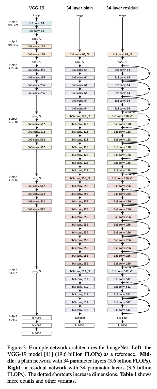
# block that's used and repeated sequentially in series is called Bottleneck block(in actual source code of ResNet i guess)
# convolutional layer are similar to linear layer, but they are used for images so they have spatial structure
# wx+b on overlapping batches of input
# for very deep networks, relu is typically more better
# basically, the general structure that is common is:
# a linear/convolutional layer
# followed by batch normalization layer
# followed by non-linearity layer eg. relu/tanh, and this repeats
# also saw use of bias=False in real world example cuz batch normalization has its own bias# torch.nn.Linear()
# a linear layer performs a wx + b, y=xA^T+b.
# to initialize we need just fan_in, fan_out so that W1 can be initialized
# in above case fan_in = n_embd * block_size, fan_out = n_hidden to let know of the matrix size
# and you can set bias=False if your linear layer is followed by a batch normalization layer
# they're using normal distribution instead of Gaussian, instead of (5/3)/fan_in, they are just using 1/fan_in and between sqr root of 1/fan_in and its -ve
# its kind of similar to what we implemented# no_of_features = 200#our case, and it is needed to initialize bngain, bnbias, bnmean_running, bnstd_running
# momentum used for running mean and running std. in docs, default is 0.1, but in our case we used 0.001 above
# for a large batch size, you can use higher momentum like 0.1
# but for our batch size = 32, mean and std might change around a lot,
# and if momentum is high eg. 0.1, it might not help our value to settle/converge to actual mean/std of entire training set
# track_running_stats determine whether or not our batch norm layer does that step in training itself to prevent calibration after training
# device: cpu, gpu
# dtype: half precision, single precision, double precisionActivation and normalization notes
# ============================================
# Lecture Summary: Activation Statistics & Batch Normalization
# ============================================

# Core idea:
# The statistics of activations and gradients are extremely important for
# training neural networks, especially as models become larger and deeper.

# Output layer:
# - Poorly scaled final activations can produce overly confident wrong predictions.
# - Confident mispredictions create very large ("hockey-stick") losses.
# - Proper initialization reduces these extreme losses, allowing training to
#   spend its effort learning instead of correcting bad initial predictions.

# Hidden layers:
# - Activations should neither collapse to 0 nor explode to very large values.
# - Extreme activations interact badly with nonlinear activation functions
#   (e.g. tanh saturation -> vanishing gradients).
# - The goal is to keep activation distributions stable across all layers.
# - Ideally, activations remain roughly Gaussian with similar scale throughout
#   the network.

# Weight initialization:
# - Properly scaling weights and biases during initialization helps maintain
#   healthy activation distributions.
# - Good initialization gives a significant improvement in optimization.

# Limitation of initialization:
# - Initialization only fixes the network at the START of training.
# - As training progresses, parameters change and activation statistics drift.
# - In very deep networks with many different layer types, carefully choosing
#   initial weights is no longer enough to keep activations well-behaved.

# Solution:
# Introduce normalization layers.

# Common normalization methods:
# - Batch Normalization (BatchNorm)
# - Layer Normalization (LayerNorm)
# - Instance Normalization
# - Group Normalization

# Batch Normalization idea:
# - Compute the batch mean and standard deviation.
# - Normalize activations to have roughly zero mean and unit variance.
# - Since normalization is differentiable, gradients can still flow normally.

# Why BatchNorm needs extra parameters:
# - Normalization alone removes the network's freedom to choose activation scale.
# - Learnable gain (gamma) restores scaling.
# - Learnable bias (beta) restores shifting.
# - The network can therefore learn the optimal distribution if needed.

# BatchNorm complication:
# - Batch statistics depend on every example in the mini-batch.
# - Therefore examples become mathematically coupled during training.
# - Hidden activations depend not only on one input but also on its batchmates.

# Inference problem:
# - During deployment we often have only one example.
# - We cannot compute meaningful batch statistics from a single sample.

# Inference solution:
# - Estimate BatchNorm mean and std from the training set (running statistics).
# - Freeze these values.
# - Use the fixed statistics during inference.

# Practical implementation:
# - Modern BatchNorm layers maintain running estimates during training.
# - This removes the need for a separate calibration step after training.

# Downsides of BatchNorm:
# - Coupling examples causes unintuitive behavior.
# - Can introduce subtle implementation bugs.
# - Has historically been a common source of debugging headaches.

# Because of these issues:
# - Many modern architectures prefer LayerNorm or GroupNorm.
# - These normalize each example independently instead of across the batch.

# Historical importance:
# - BatchNorm (introduced around 2015) was a breakthrough.
# - It made training much deeper neural networks reliable.
# - Its main contribution was controlling activation statistics throughout
#   the network, leading to faster and more stable optimization.

# Looking ahead:
# - Future topics (e.g. Recurrent Neural Networks) are effectively extremely
#   deep networks when unrolled through time.
# - Keeping activations and gradients stable becomes even more critical there.
# - Understanding initialization, activation statistics, and normalization is
#   fundamental for successfully training deep neural networks.
Layers and diagnostic plots
# pytorch-ifying the code, continue from 1:09:29# torch.nn.Linear is a fully connected layer that computes:
# y = W @ x + b
# where W (weights) and b (bias) are learnable parameters.
# fan_in = number of input features
# fan_out = number of output features
# Weights are initialized using Kaiming initialization (good default for deep nets).
# Biases are typically initialized to zeros.
# layer.parameters() returns only the learnable parameters (weight and bias).
# BatchNorm1d(num_features, eps, momentum)
# eps: small value added to avoid division by zero.
# momentum: controls how quickly running statistics are updated.
# BatchNorm behaves differently during training and inference.
# During training:
# - Normalize using the current batch's mean and variance.
# - Update running_mean and running_var.
# During inference (evaluation):
# - Normalize using the stored running_mean and running_var.
# - Do NOT update the running statistics.
# gamma (weight) and beta (bias) are learnable parameters.
# running_mean and running_var are buffers (not optimized by gradient descent).
# Buffers are updated manually using an Exponential Moving Average (EMA),
# so they are not returned by layer.parameters().
# The BatchNorm paper stores running VARIANCE (std^2), not running standard deviation.
# layer.out is NOT part of PyTorch.
# Karpathy adds it only to save activations for plotting and debugging.
# torch.no_grad() is used when updating running_mean/running_var because
# these updates should not be tracked by autograd or included in backpropagation.
# Tanh layer simply computes:
# y = tanh(x)
# It has no learnable parameters.
# Representing everything as layers (Linear, BatchNorm, Tanh) lets us:
# - stack them easily,
# - loop through them,
# - collect all parameters automatically.
# Gain is adjusted during initialization to help control activation statistics,
# especially in deeper networks.
# Nested list comprehension collects parameters from every layer:
# [p for layer in layers for p in layer.parameters()]
# retain_grad() tells PyTorch to keep gradients for intermediate activations.
# Normally, gradients are only stored for leaf tensors (model parameters).
# Karpathy keeps them to inspect and plot gradient statistics.# Let's train a deeper network
class Linear:
def __init__(self, fan_in, fan_out, bias=True):
self.weight = torch.randn((fan_in, fan_out), generator=g) / fan_in**0.5
self.bias = torch.zeros(fan_out) if bias else None
def __call__(self, x):
self.out = x @ self.weight
if self.bias is not None:
self.out += self.bias
return self.out
def parameters(self):
return [self.weight] + ([] if self.bias is None else [self.bias])
class BatchNorm1d:
def __init__(self, dim, eps=1e-5, momentum = 0.1):
self.eps = eps
self.momentum = momentum
self.training = True
# parameters(trained with backprop)
self.gamma = torch.ones(dim)
self.beta = torch.zeros(dim)
# buffers (trained with a running 'momentum update')
self.running_mean = torch.zeros(dim)
self.running_var = torch.ones(dim)
def __call__(self, x):
# calculate the forward pass
if self.training:
xmean = x.mean(0, keepdim=True) #batch mean
xvar = x.var(0, keepdim=True, unbiased=True) #batch variance
else:
xmean = self.running_mean
xvar = self.running_var
xhat = (x - xmean) / torch.sqrt(xvar + self.eps) #normalize to unit variance
self.out = self.gamma * xhat + self.beta
# update the buffers
if self.training:
with torch.no_grad():
self.running_mean = (1 - self.momentum) * self.running_mean + self.momentum * xmean
self.running_var = (1 - self.momentum) * self.running_var + self.momentum * xvar
return self.out
def parameters(self):
return [self.gamma, self.beta]
class Tanh:
def __call__(self, x):
self.out = torch.tanh(x)
return self.out
def parameters(self):
return []
n_embd = 10 #dimensionality of character embedding vectors
n_hidden = 100 #number of neurons in hidden layer of MLP
g = torch.Generator().manual_seed(2147483647) #for reproducibility
C = torch.randn((vocab_size, n_embd), generator=g)
layers = [
Linear(n_embd * block_size, n_hidden), Tanh(),
Linear(n_hidden, n_hidden), Tanh(),
Linear(n_hidden, n_hidden), Tanh(),
Linear(n_hidden, n_hidden), Tanh(),
Linear(n_hidden, n_hidden), Tanh(),
Linear(n_hidden, vocab_size),
]
with torch.no_grad():
# last layer: make less confident
layers[-1].weight *= 0.1
# all other layers: apply gain
for layer in layers[:-1]:
if isinstance(layer, Linear):
layer.weight *= 5/3 #1
parameters = [C] + [p for layer in layers for p in layer.parameters()]
print(sum(p.nelement() for p in parameters)) # no of parameters in total
for p in parameters:
p.requires_grad = True46497
# same optimization as previously done
max_steps = 200000
batch_size = 32
lossi = []
ud = []

for i in range(max_steps):

    # minibatch construct
    ix = torch.randint(0, Xtr.shape[0], (batch_size, ), generator = g)
    Xb, Yb = Xtr[ix], Ytr[ix] #batch X, Y

    # forward pass
    emb = C[Xb] #embed the characters into vectors
    x = emb.view(emb.shape[0], -1) #concatenate the vectors

    for layer in layers:
        x = layer(x)
    loss = F.cross_entropy(x, Yb) #loss function

    # backward pass
    for layer in layers:
        layer.out.retain_grad() #after debug: would take out retain grad
    for p in parameters:
        p.grad = None
    loss.backward()

    # update
    lr = 0.1 if i < 100000 else 0.01 # step learning rate decay
    for p in parameters:
        p.data += -lr * p.grad

    # track stats
    if i % 10000 == 0: #print every once in a while
        print(f'{i:7d}/{max_steps:7d}: {loss.item():.4f}')
    lossi.append(loss.log10().item())
    with torch.no_grad():
        ud.append([((lr*p.grad).std() / p.data.std()).log10().item() for p in parameters])

    if i >= 1000: #for the last 2 graphs, need to go through more iterations
        break #after first iteration itself, obviously remove this after debug
0/ 200000: 3.2962
# activation statistics in forward pass(if gain set to 1 instead of 5/3)

# visualize histograms of forward pass activations specifically at tanh layers
plt.figure(figsize=(20,4)) #width and height of the plot
legends = []

for i, layer in enumerate(layers[:-1]): #while iterating over all layer,s exclude only the output softmax layer
    if isinstance(layer, Tanh): #tanh cuz they have finite output -1 to +1, easy to visualize
        t = layer.out
        # we define saturation as > 0.97, which is tail of tanh, and it stops gradients
        print('layer %d (%10s): mean %+.2f, std %.2f, saturated: %.2f%%' % (i, layer.__class__.__name__, t.mean(), t.std(), (t.abs() > 0.97).float().mean()*100))
        hy, hx = torch.histogram(t, density=True)
        plt.plot(hx[:-1].detach(), hy.detach())
        legends.append(f'layer {i} ( {layer.__class__.__name__}')
plt.legend(legends);
plt.title('activation distribution')
layer 1 ( Tanh): mean -0.02, std 0.62, saturated: 3.50%
layer 3 ( Tanh): mean -0.00, std 0.48, saturated: 0.03%
layer 5 ( Tanh): mean +0.00, std 0.41, saturated: 0.06%
layer 7 ( Tanh): mean +0.00, std 0.35, saturated: 0.00%
layer 9 ( Tanh): mean -0.02, std 0.32, saturated: 0.00%
Text(0.5, 1.0, 'activation distribution')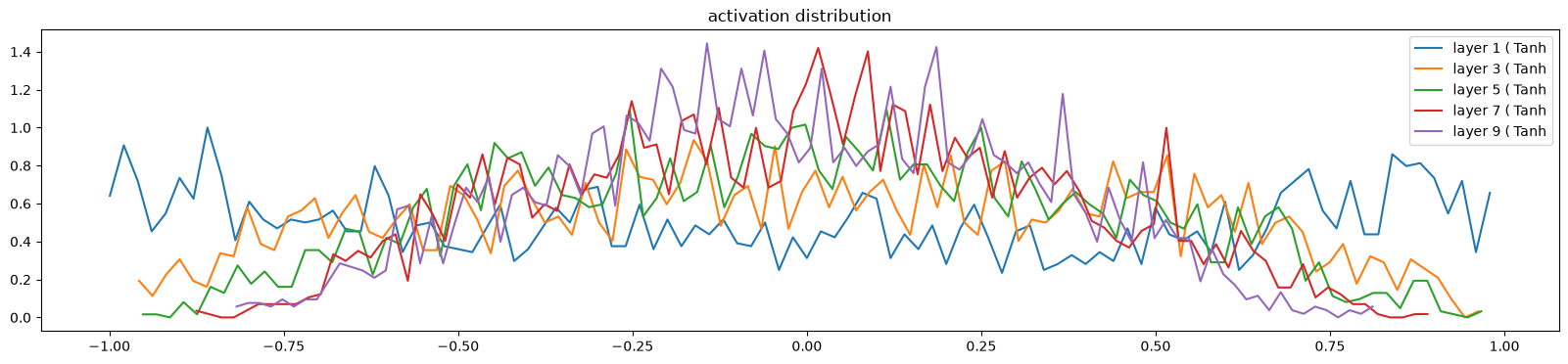
# Visualize the FORWARD activations (outputs) of each tanh layer.

# We only inspect tanh layers because:
# - tanh outputs are bounded in [-1, 1], making them easy to visualize.
# - Saturation (outputs near ±1) is also easy to detect.

# For each tanh layer:
# - Compute the mean and standard deviation of its activations.
# - Compute the % of saturated neurons.

# Saturation is defined as:
# abs(tanh_output) > 0.97
# These neurons lie in the flat tails of tanh, where gradients nearly vanish.

# Plot a histogram of activations to see their distribution.
# Ideally, activations should be centered around 0 and not pile up near ±1.


# With gain = 5/3:
# - Activation distributions remain stable across layers.
# - Standard deviation stays roughly constant (~0.65).
# - Only about 5% of neurons are saturated.
# - This is a healthy operating point for tanh networks.


# Gain is applied after Kaiming initialization:
# weight *= gain
# It compensates for tanh shrinking (squashing) the activations.


# Without the gain (gain = 1):
# - Every tanh layer slightly shrinks the activations.
# - Standard deviation decreases layer by layer.
# - Activations slowly collapse toward 0.
# - Very little saturation occurs, but the signal becomes weaker.


# With too large a gain (e.g. gain = 3):
# - Activations become too large.
# - Many neurons saturate at ±1.
# - Too much saturation leads to vanishing gradients.


# Gain = 5/3 empirically balances these two extremes:
# - Prevents activations from shrinking.
# - Avoids excessive saturation.
# - Keeps activation statistics roughly constant across deep tanh networks.


# Karpathy notes:
# He doesn't know the exact mathematical derivation of 5/3,
# but empirically it works very well for Linear -> tanh -> Linear -> tanh networks.
# activation statistics in forward pass(if gain set to 5/3)
# visualize histograms of forward pass activations specifically at tanh layers
plt.figure(figsize=(20,4)) #width and height of the plot
legends = []
for i, layer in enumerate(layers[:-1]): #while iterating over all layer,s exclude only the output softmax layer
if isinstance(layer, Tanh): #tanh cuz they have finite output -1 to +1, easy to visualize
t = layer.out
# we define saturation as > 0.97, which is tail of tanh, and it stops gradients
print('layer %d (%10s): mean %+.2f, std %.2f, saturated: %.2f%%' % (i, layer.__class__.__name__, t.mean(), t.std(), (t.abs() > 0.97).float().mean()*100))
hy, hx = torch.histogram(t, density=True)
plt.plot(hx[:-1].detach(), hy.detach())
legends.append(f'layer {i} ( {layer.__class__.__name__}')
plt.legend(legends);
plt.title('activation distribution')layer 1 ( Tanh): mean -0.04, std 0.76, saturated: 21.97%
layer 3 ( Tanh): mean -0.01, std 0.72, saturated: 11.00%
layer 5 ( Tanh): mean +0.01, std 0.73, saturated: 13.00%
layer 7 ( Tanh): mean -0.05, std 0.73, saturated: 13.34%
layer 9 ( Tanh): mean +0.00, std 0.72, saturated: 10.53%
Text(0.5, 1.0, 'activation distribution')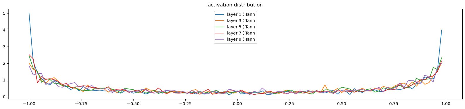
# in the case above, if we have more layers, it will stabilize at around 0.65 and saturation will be roughly 5%
# why does this stabilize and give us a nice distribution? cuz gain = 5/3
# std shrinks and saturation comes to 0# activation statistics in backward pass
# visualize histograms
plt.figure(figsize=(20,4)) #width and height of the plot
legends = []
for i, layer in enumerate(layers[:-1]): #exclude the output layer
if isinstance(layer, Tanh):
t = layer.out.grad
print('layer %d (%10s): mean %+f, std %e' % (i, layer.__class__.__name__, t.mean(), t.std()))
hy, hx = torch.histogram(t, density=True)
plt.plot(hx[:-1].detach(), hy.detach())
legends.append(f'layer {i} {layer.__class__.__name__}')
plt.legend(legends);
plt.title('activation distribution')layer 1 ( Tanh): mean +0.000024, std 3.353992e-03
layer 3 ( Tanh): mean +0.000012, std 3.157344e-03
layer 5 ( Tanh): mean -0.000004, std 2.925863e-03
layer 7 ( Tanh): mean +0.000036, std 2.715700e-03
layer 9 ( Tanh): mean +0.000020, std 2.308167e-03
Text(0.5, 1.0, 'activation distribution')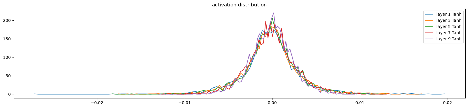
# in graph above, we're looking that all layers have roughly the same gradient
# things are not shrinking or exploding# what happens if you comment out all tanh non-linearities, but keep everything else: eg. gain of 5/3 ,etc
# in visualization, you have to replace Tanh with Linear
# basically, what happens is that there will be rapid shrinking with no tanh fighting it back# but why do we need tanh? why not just a stack of linear layers and just set gain = 1, it is also well behaved right(experiment if you want).
# but it is just a big linear sandwich and it collapses into a single layer in terms of representation power
# so, no matter how many layers you add, at the end you get just a linear transformation, it will just be the same Wx + b but with bigger w and b's
# i.e. its equivalent to using single layer if we don't use non-linearity like tanh
# so basically, tanh non-linearities allows us to turn this linear function into a neural net that can approximate any arbitrary function# getting neural nets to train before these advanced optimizers like adam, residual connections was like balancing pencil on finger
# you had to carefully orchestrate everything, be very wary of precision of activations, gradients, statistics
# it was impossible to train very deep networks cuz you'd have to be very careful with initialization# plots personally used by andrej to debug neural networks# ============================================================
# Viz #3: Parameter Statistics
# ============================================================
# Analyze the model parameters (weights) and their gradients.
# Only weight matrices (2D tensors) are plotted.
# Biases and BatchNorm gamma/beta are skipped for simplicity.
# For each weight matrix:
# - Compute mean and standard deviation.
# - Plot a histogram of parameter values.
# - Compute the gradient-to-data ratio.
# Gradient-to-data ratio:
# std(grad) / std(weight)
#
# Measures how large the gradients are compared to the parameter values.
# If gradients are too large, parameter updates become unstable.
# If gradients are too small, learning becomes very slow.
# Ideally, gradients should be much smaller than the weights.
# Here they are roughly 1000x smaller (ratio ≈ 1e-3), which is reasonable.
# Observation:
# The final output layer is an outlier.
# Its gradients are about 10x larger than the other layers,
# meaning SGD updates this layer much faster initially.
# This happens because the final layer was intentionally initialized
# with smaller weights to make the initial softmax less confident.
# After some training (e.g. 1000 iterations),
# this imbalance mostly corrects itself as the weights adapt.# visualize histograms
plt.figure(figsize=(20, 4)) # width and height of the plot
legends = []
for i,p in enumerate(parameters):
t = p.grad
if p.ndim == 2:
print('weight %10s | mean %+f | std %e | grad:data ratio %e' % (tuple(p.shape), t.mean(), t.std(), t.std() / p.std()))
hy, hx = torch.histogram(t, density=True)
plt.plot(hx[:-1].detach(), hy.detach())
legends.append(f'{i} {tuple(p.shape)}')
plt.legend(legends)
plt.title('weights gradient distribution');weight (27, 10) | mean +0.000980 | std 1.189171e-02 | grad:data ratio 1.189149e-02
weight (30, 100) | mean +0.000118 | std 1.005291e-02 | grad:data ratio 3.214556e-02
weight (100, 100) | mean +0.000033 | std 7.821212e-03 | grad:data ratio 4.653362e-02
weight (100, 100) | mean -0.000107 | std 6.655620e-03 | grad:data ratio 3.925851e-02
weight (100, 100) | mean -0.000017 | std 6.086041e-03 | grad:data ratio 3.605768e-02
weight (100, 100) | mean -0.000077 | std 5.075620e-03 | grad:data ratio 3.015269e-02
weight (100, 27) | mean -0.000000 | std 2.056585e-02 | grad:data ratio 2.909910e-01
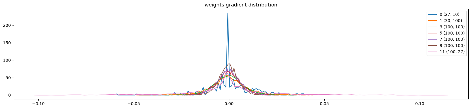
# ============================================================
# Viz #4: Update-to-Data Ratio
# ============================================================
# Gradient-to-data ratio isn't the whole story.
# The actual parameter update is:
#
# update = learning_rate * gradient
#
# So what really matters is:
#
# std(update) / std(weight)
# This measures how much each parameter changes every iteration
# relative to its current magnitude.
# Karpathy plots:
# log10(std(update) / std(weight))
#
# Using log10 makes it easy to compare values across layers.
# Ideal update ratio:
# around 1e-3 (log10 ≈ -3)
# Interpretation:
# log10 ≈ -3
# -> parameters change by about 0.1% each step (healthy)
# Much larger (e.g. -1):
# -> updates are too large
# -> training may become unstable
# Much smaller (e.g. -4 or lower):
# -> updates are tiny
# -> learning is too slow
# The final layer starts above the others because its weights were
# artificially shrunk during initialization.
# As training progresses, it gradually stabilizes.
# This plot is also useful for tuning the learning rate.
# Example:
# If learning rate = 0.001,
# all update ratios become much smaller than -3,
# indicating that training is unnecessarily slow.
# If update ratios are slightly above -3 (e.g. around -2.5),
# learning is a bit aggressive but often still reasonable.plt.figure(figsize=(20, 4))
legends = []
for i,p in enumerate(parameters):
if p.ndim == 2:
plt.plot([ud[j][i] for j in range(len(ud))])
legends.append('param %d' % i)
plt.plot([0, len(ud)], [-3, -3], 'k') # these ratios should be ~1e-3, indicate on plot
plt.legend(legends);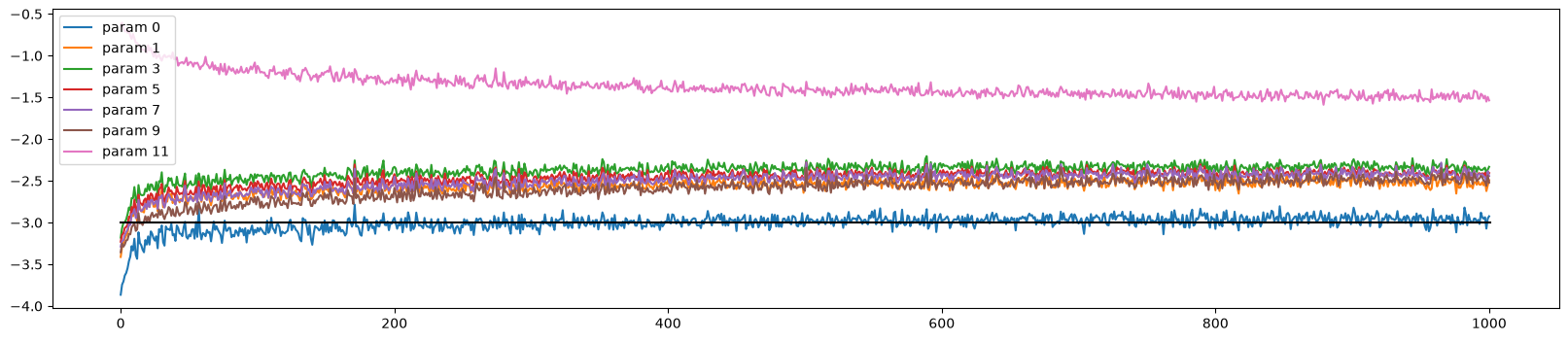
# ============================================================
# Debugging with these plots
# ============================================================
# Properly initialized networks should show:
# - Stable activation distributions.
# - Stable gradient distributions.
# - Reasonable parameter histograms.
# - Update ratios around 1e-3.
# If initialization is wrong (e.g. no fan-in scaling):
# - Activations become heavily saturated.
# - Gradients become poorly distributed.
# - Parameter histograms become irregular.
# - Different layers learn at very different speeds.
# - Update ratios become much larger than expected.
# These visualization plots quickly reveal
# whether a network is well-calibrated or miscalibrated,
# making them powerful debugging tools during training.# until now, it feels like balancing a pencil on a finger, now we introduce batch normalization
# typical place to put batch normalization is between linear layer and non-linearity
# but you can get similar results even if you place if after tanh
# its fine to place it at end after last linear layer and before the loss function# Let's train a deeper network
class Linear:
def __init__(self, fan_in, fan_out, bias=True):
self.weight = torch.randn((fan_in, fan_out), generator=g) / fan_in**0.5
self.bias = torch.zeros(fan_out) if bias else None
def __call__(self, x):
self.out = x @ self.weight
if self.bias is not None:
self.out += self.bias
return self.out
def parameters(self):
return [self.weight] + ([] if self.bias is None else [self.bias])
class BatchNorm1d:
def __init__(self, dim, eps=1e-5, momentum = 0.1):
self.eps = eps
self.momentum = momentum
self.training = True
# parameters(trained with backprop)
self.gamma = torch.ones(dim)
self.beta = torch.zeros(dim)
# buffers (trained with a running 'momentum update')
self.running_mean = torch.zeros(dim)
self.running_var = torch.ones(dim)
def __call__(self, x):
# calculate the forward pass
if self.training:
xmean = x.mean(0, keepdim=True) #batch mean
xvar = x.var(0, keepdim=True, unbiased=True) #batch variance
else:
xmean = self.running_mean
xvar = self.running_var
xhat = (x - xmean) / torch.sqrt(xvar + self.eps) #normalize to unit variance
self.out = self.gamma * xhat + self.beta
# update the buffers
if self.training:
with torch.no_grad():
self.running_mean = (1 - self.momentum) * self.running_mean + self.momentum * xmean
self.running_var = (1 - self.momentum) * self.running_var + self.momentum * xvar
return self.out
def parameters(self):
return [self.gamma, self.beta]
class Tanh:
def __call__(self, x):
self.out = torch.tanh(x)
return self.out
def parameters(self):
return []
n_embd = 10 #dimensionality of character embedding vectors
n_hidden = 100 #number of neurons in hidden layer of MLP
g = torch.Generator().manual_seed(2147483647) #for reproducibility
C = torch.randn((vocab_size, n_embd), generator=g)
layers = [
Linear(n_embd * block_size, n_hidden), BatchNorm1d(n_hidden), Tanh(),
Linear(n_hidden, n_hidden), BatchNorm1d(n_hidden), Tanh(),
Linear(n_hidden, n_hidden), BatchNorm1d(n_hidden), Tanh(),
Linear(n_hidden, n_hidden), BatchNorm1d(n_hidden), Tanh(),
Linear(n_hidden, n_hidden), BatchNorm1d(n_hidden), Tanh(),
Linear(n_hidden, vocab_size), BatchNorm1d(vocab_size),
]
with torch.no_grad():
# last layer: make less confident
# layers[-1].weight *= 0.1
# since the last layer is batchnorm, we won't change the weight to make the softmax less confident
# we'll change gamma: variable that multiplicatively interacts with output of normalization
layers[-1].gamma *= 0.1
# all other layers: apply gain
for layer in layers[:-1]:
if isinstance(layer, Linear):
layer.weight *= 5/3 #1
parameters = [C] + [p for layer in layers for p in layer.parameters()]
print(sum(p.nelement() for p in parameters)) # no of parameters in total
for p in parameters:
p.requires_grad = True47551
# same optimization as previously done
max_steps = 200000
batch_size = 32
lossi = []
ud = []
for i in range(max_steps):
# minibatch construct
ix = torch.randint(0, Xtr.shape[0], (batch_size, ), generator = g)
Xb, Yb = Xtr[ix], Ytr[ix] #batch X, Y
# forward pass
emb = C[Xb] #embed the characters into vectors
x = emb.view(emb.shape[0], -1) #concatenate the vectors
for layer in layers:
x = layer(x)
loss = F.cross_entropy(x, Yb) #loss function
# backward pass
for layer in layers:
layer.out.retain_grad() #after debug: would take out retain grad
for p in parameters:
p.grad = None
loss.backward()
# update
lr = 0.1 if i < 100000 else 0.01 # step learning rate decay
for p in parameters:
p.data += -lr * p.grad
# track stats
if i % 10000 == 0: #print every once in a while
print(f'{i:7d}/{max_steps:7d}: {loss.item():.4f}')
lossi.append(loss.log10().item())
with torch.no_grad():
ud.append([((lr*p.grad).std() / p.data.std()).log10().item() for p in parameters])
if i >= 1000: #for the last 2 graphs, need to go through more iterations
break #after first iteration itself, obviously remove this after debug 0/ 200000: 3.2870
# this looks really good, cuz of normalization of batch before every tanh
# std is roughly 0.65, saturation 2%, and roughly equal s.d. throughout the entire layers
# lol, so we had forgotten to put batch normalization for first layer, and it was so weird and different from others
# activation statistics in forward pass(if gain set to 5/3)

# visualize histograms of forward pass activations specifically at tanh layers
plt.figure(figsize=(20,4)) #width and height of the plot
legends = []

for i, layer in enumerate(layers[:-1]): #while iterating over all layer,s exclude only the output softmax layer
    if isinstance(layer, Tanh): #tanh cuz they have finite output -1 to +1, easy to visualize
        t = layer.out
        # we define saturation as > 0.97, which is tail of tanh, and it stops gradients
        print('layer %d (%10s): mean %+.2f, std %.2f, saturated: %.2f%%' % (i, layer.__class__.__name__, t.mean(), t.std(), (t.abs() > 0.97).float().mean()*100))
        hy, hx = torch.histogram(t, density=True)
        plt.plot(hx[:-1].detach(), hy.detach())
        legends.append(f'layer {i} ( {layer.__class__.__name__}')
plt.legend(legends);
plt.title('activation distribution')
layer 2 ( Tanh): mean -0.00, std 0.63, saturated: 2.62%
layer 5 ( Tanh): mean +0.00, std 0.64, saturated: 2.47%
layer 8 ( Tanh): mean -0.00, std 0.64, saturated: 2.16%
layer 11 ( Tanh): mean +0.00, std 0.65, saturated: 1.81%
layer 14 ( Tanh): mean -0.00, std 0.65, saturated: 1.78%
Text(0.5, 1.0, 'activation distribution')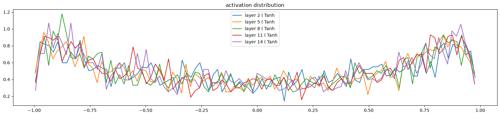
# activation statistics in backward pass

# visualize histograms
plt.figure(figsize=(20,4)) #width and height of the plot
legends = []

for i, layer in enumerate(layers[:-1]): #exclude the output layer
    if isinstance(layer, Tanh):
        t = layer.out.grad
        print('layer %d (%10s): mean %+f, std %e' % (i, layer.__class__.__name__, t.mean(), t.std()))
        hy, hx = torch.histogram(t, density=True)
        plt.plot(hx[:-1].detach(), hy.detach())
        legends.append(f'layer {i} {layer.__class__.__name__}')
plt.legend(legends);
plt.title('activation distribution')
layer 2 ( Tanh): mean -0.000000, std 3.682961e-03
layer 5 ( Tanh): mean -0.000000, std 3.262612e-03
layer 8 ( Tanh): mean +0.000000, std 2.973734e-03
layer 11 ( Tanh): mean +0.000000, std 2.741114e-03
layer 14 ( Tanh): mean +0.000000, std 2.584295e-03
Text(0.5, 1.0, 'activation distribution')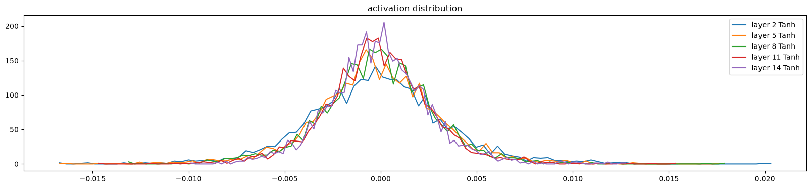
# visualize histograms
plt.figure(figsize=(20, 4)) # width and height of the plot
legends = []
for i,p in enumerate(parameters):
  t = p.grad
  if p.ndim == 2:
    print('weight %10s | mean %+f | std %e | grad:data ratio %e' % (tuple(p.shape), t.mean(), t.std(), t.std() / p.std()))
    hy, hx = torch.histogram(t, density=True)
    plt.plot(hx[:-1].detach(), hy.detach())
    legends.append(f'{i} {tuple(p.shape)}')
plt.legend(legends)
plt.title('weights gradient distribution');
weight (27, 10) | mean +0.000000 | std 1.019890e-02 | grad:data ratio 1.018851e-02
weight (30, 100) | mean +0.000092 | std 8.238448e-03 | grad:data ratio 2.635845e-02
weight (100, 100) | mean +0.000031 | std 7.318127e-03 | grad:data ratio 4.377153e-02
weight (100, 100) | mean -0.000019 | std 6.662029e-03 | grad:data ratio 3.949899e-02
weight (100, 100) | mean -0.000019 | std 5.821521e-03 | grad:data ratio 3.468164e-02
weight (100, 100) | mean +0.000053 | std 5.445303e-03 | grad:data ratio 3.243371e-02
weight (100, 27) | mean -0.000165 | std 1.046846e-02 | grad:data ratio 6.281275e-02
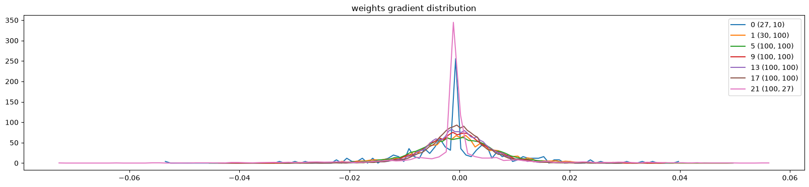
plt.figure(figsize=(20, 4))
legends = []
for i,p in enumerate(parameters):
  if p.ndim == 2:
    plt.plot([ud[j][i] for j in range(len(ud))])
    legends.append('param %d' % i)
plt.plot([0, len(ud)], [-3, -3], 'k') # these ratios should be ~1e-3, indicate on plot
plt.legend(legends);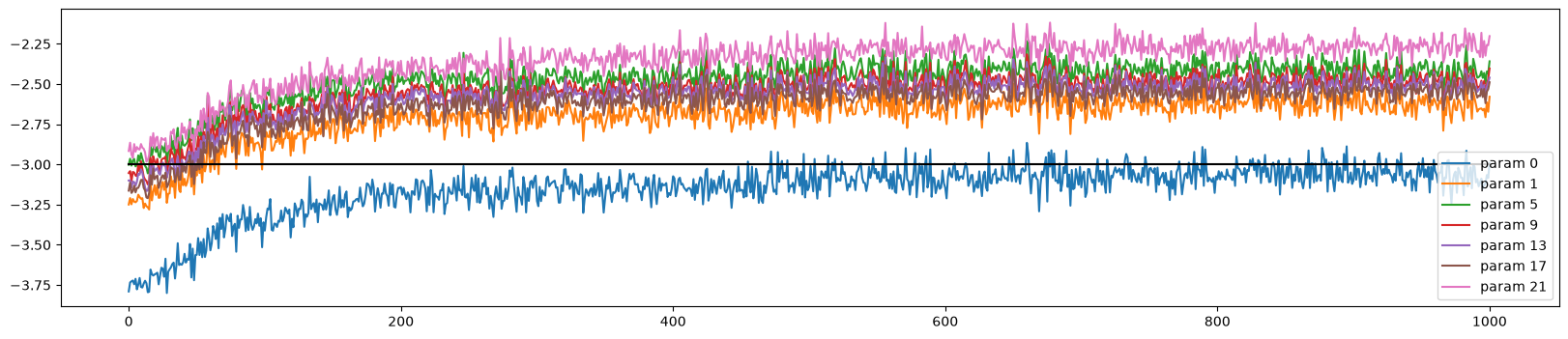
# we're going above -3 a little bit, but not by too much
# all parameters are training at roughly the same rate# now if you replace gain 5/3 with eg. 0.2, it will almost have 0 effect cuz of batch normalization and everything looks the same
# except of course the the updates at last graph
# even though the forward and backward pass look okay
# because of backward pass of batch norm and the scale of incoming activations interacts in the batchnorm and its backward pass
# this is changing the scale of the updates on these parameters
# so the gradients on the weights are affected
# so we still don't have the luxury to not use non-arbitrary gain 5/3, but everything else is significantly more robust
# that last graph's special case of arbitrary gain initialization is not shown here, you can test it if u wish# and when we use batchnorm, we don't even have to normalize by fan_in sometimes, where we divided by fan_in ** 0.5
# remove it and see that because of batchnorm, it will behave relatively well, though little bit not preferred# we can change the gain, but if we do so, we have to worry a little about the update scales
# and making sure that learning rate is properly calibratedLessons from normalization
# summary:
# introduced batchnorm: stabilize very deep neural networks and their training
# pytorchify our code and wrap up into modules: Linear, BatchNorm1D, Tanh which can be stacked up into neural nets like lego building blocks
# these layers actually exist in pytorch, and if you import torch.nn
# you can just replace above code, eg. Linear with nn.Linear, and it will work
# cuz the api we built here is identical to the api that pytorch uses
# our implementation is also identical to that of pytorch
# understood diagnostic tools we can use to understand whether our neural network is in a good state dynamically
# looking at statistics, histograms and activations of forward pass activations, backward pass gradients,
# the weights that are going to be updated as part of stochastic gradient descent, their means, sd, ratio of gradients to data
# and the last graph: updates to data, not look at single iteration of time, but growth over time
# and log(-3) is a good rough heuristic for what we want the ratio to be on that last graph
# if its very high, then the learning rate or the updates are too big, and same for small case# we tried to beat the previous performance using batchnorm layer but it didn't work, cuz that isn't the bottle neck right now
# that was alternatively optimized by initializing the weights properly
# we suspect that the bottleneck is the context length of our context. we're just taking 3 characters to predict the 4th,
# and we need to go beyond that
# and we need to look at more powerful architectures like recurrent neural networks and transformers to push the loss probabilities we are getting on this dataset# i want to see outputs# same optimization as previously done
max_steps = 200000
batch_size = 32
lossi = []
ud = []
for i in range(max_steps):
# minibatch construct
ix = torch.randint(0, Xtr.shape[0], (batch_size, ), generator = g)
Xb, Yb = Xtr[ix], Ytr[ix] #batch X, Y
# forward pass
emb = C[Xb] #embed the characters into vectors
x = emb.view(emb.shape[0], -1) #concatenate the vectors
for layer in layers:
x = layer(x)
loss = F.cross_entropy(x, Yb) #loss function
# backward pass
for layer in layers:
layer.out.retain_grad() #after debug: would take out retain grad
for p in parameters:
p.grad = None
loss.backward()
# update
lr = 0.1 if i < 100000 else 0.01 # step learning rate decay
for p in parameters:
p.data += -lr * p.grad
# track stats
if i % 10000 == 0: #print every once in a while
print(f'{i:7d}/{max_steps:7d}: {loss.item():.4f}')
lossi.append(loss.log10().item())
with torch.no_grad():
ud.append([((lr*p.grad).std() / p.data.std()).log10().item() for p in parameters]) 0/ 200000: 3.2870
10000/ 200000: 2.3578
20000/ 200000: 2.1042
30000/ 200000: 1.9646
40000/ 200000: 2.2145
50000/ 200000: 2.2262
60000/ 200000: 1.7340
70000/ 200000: 2.1743
80000/ 200000: 2.1895
90000/ 200000: 1.8283
100000/ 200000: 2.3646
110000/ 200000: 2.2026
120000/ 200000: 2.1039
130000/ 200000: 1.8566
140000/ 200000: 1.8049
150000/ 200000: 1.9258
160000/ 200000: 1.8757
170000/ 200000: 1.8330
180000/ 200000: 2.2324
190000/ 200000: 2.0522
# visualize histograms
plt.figure(figsize=(20, 4)) # width and height of the plot
legends = []
for i, layer in enumerate(layers[:-1]): # note: exclude the output layer
if isinstance(layer, Tanh):
t = layer.out
print('layer %d (%10s): mean %+.2f, std %.2f, saturated: %.2f%%' % (i, layer.__class__.__name__, t.mean(), t.std(), (t.abs() > 0.97).float().mean()*100))
hy, hx = torch.histogram(t, density=True)
plt.plot(hx[:-1].detach(), hy.detach())
legends.append(f'layer {i} ({layer.__class__.__name__}')
plt.legend(legends);
plt.title('activation distribution')layer 2 ( Tanh): mean -0.01, std 0.69, saturated: 14.06%
layer 5 ( Tanh): mean -0.02, std 0.72, saturated: 16.84%
layer 8 ( Tanh): mean -0.00, std 0.75, saturated: 15.81%
layer 11 ( Tanh): mean +0.02, std 0.77, saturated: 16.75%
layer 14 ( Tanh): mean -0.02, std 0.79, saturated: 18.91%
Text(0.5, 1.0, 'activation distribution')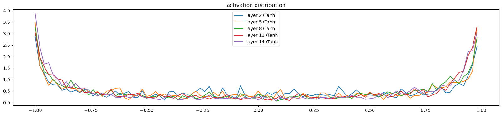
# visualize histograms
plt.figure(figsize=(20, 4)) # width and height of the plot
legends = []
for i, layer in enumerate(layers[:-1]): # note: exclude the output layer
if isinstance(layer, Tanh):
t = layer.out.grad
print('layer %d (%10s): mean %+f, std %e' % (i, layer.__class__.__name__, t.mean(), t.std()))
hy, hx = torch.histogram(t, density=True)
plt.plot(hx[:-1].detach(), hy.detach())
legends.append(f'layer {i} ({layer.__class__.__name__}')
plt.legend(legends);
plt.title('gradient distribution')layer 2 ( Tanh): mean -0.000000, std 3.421682e-03
layer 5 ( Tanh): mean -0.000000, std 3.288253e-03
layer 8 ( Tanh): mean -0.000000, std 3.270637e-03
layer 11 ( Tanh): mean -0.000000, std 3.539113e-03
layer 14 ( Tanh): mean -0.000000, std 3.846485e-03
Text(0.5, 1.0, 'gradient distribution')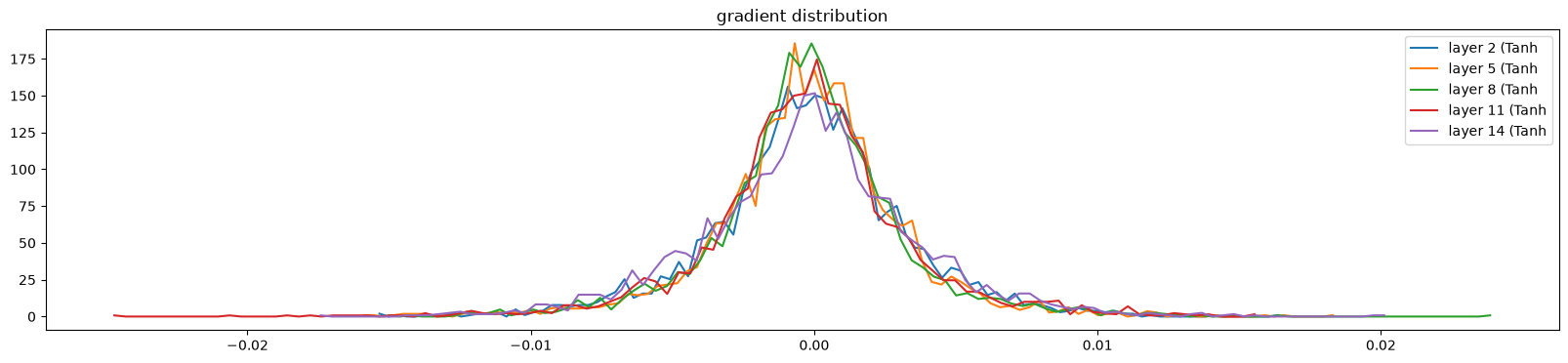
# visualize histograms
plt.figure(figsize=(20, 4)) # width and height of the plot
legends = []
for i,p in enumerate(parameters):
  t = p.grad
  if p.ndim == 2:
    print('weight %10s | mean %+f | std %e | grad:data ratio %e' % (tuple(p.shape), t.mean(), t.std(), t.std() / p.std()))
    hy, hx = torch.histogram(t, density=True)
    plt.plot(hx[:-1].detach(), hy.detach())
    legends.append(f'{i} {tuple(p.shape)}')
plt.legend(legends)
plt.title('weights gradient distribution');
weight (27, 10) | mean +0.000000 | std 1.496443e-02 | grad:data ratio 1.370268e-02
weight (30, 100) | mean +0.000084 | std 7.878289e-03 | grad:data ratio 1.922244e-02
weight (100, 100) | mean +0.000060 | std 5.057851e-03 | grad:data ratio 2.049041e-02
weight (100, 100) | mean -0.000087 | std 5.180276e-03 | grad:data ratio 2.133905e-02
weight (100, 100) | mean +0.000043 | std 5.201565e-03 | grad:data ratio 2.196100e-02
weight (100, 100) | mean -0.000013 | std 5.238893e-03 | grad:data ratio 2.278768e-02
weight (100, 27) | mean +0.000054 | std 9.173456e-03 | grad:data ratio 2.777520e-02
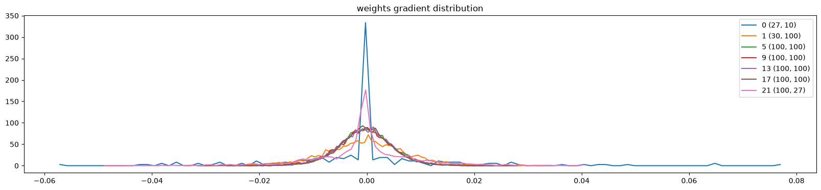
plt.figure(figsize=(20, 4))
legends = []
for i,p in enumerate(parameters):
  if p.ndim == 2:
    plt.plot([ud[j][i] for j in range(len(ud))])
    legends.append('param %d' % i)
plt.plot([0, len(ud)], [-3, -3], 'k') # these ratios should be ~1e-3, indicate on plot
plt.legend(legends);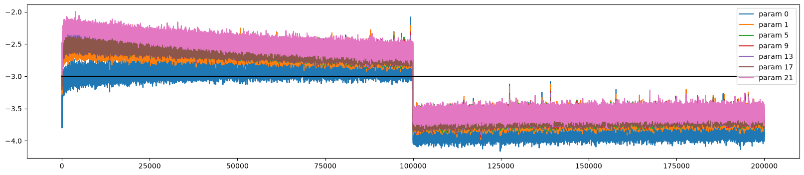
@torch.no_grad() # this decorator disables gradient tracking
def split_loss(split):
  x,y = {
    'train': (Xtr, Ytr),
    'val': (Xdev, Ydev),
    'test': (Xte, Yte),
  }[split]
  emb = C[x] # (N, block_size, n_embd)
  x = emb.view(emb.shape[0], -1) # concat into (N, block_size * n_embd)
  for layer in layers:
    x = layer(x)
  loss = F.cross_entropy(x, y)
  print(split, loss.item())

# put layers into eval mode
for layer in layers:
  layer.training = False
split_loss('train')
split_loss('val')
train 2.012324094772339
val 2.084045648574829
# previous loss log:
train 2.1270017623901367
val 2.169905662536621
# previous loss log:
train 2.069589138031006
val 2.1310746669769287
# previous loss log
train 2.0355966091156006
val 2.1026785373687744
# previous loss log
train 2.0376641750335693
val 2.106989622116089
# previous loss log
train 2.0668270587921143
val 2.104844808578491
# previous loss log
train 2.0668270587921143
val 2.1049270629882812
# previous loss log
train 2.06659197807312
val 2.1050572395324707
# current final loss log after implementing batch norm too
# (won't be much diff cuz weights were initialized nicely before too which is good alternative but difficult to do in deep neural nets
train 2.012324094772339
val 2.084045648574829Further experiments
emb.shapetorch.Size([3, 10])# sample from the model
g = torch.Generator().manual_seed(2147483647 + 10)
for _ in range(20):
out = []
context = [0] * block_size #initialize with all ...
while True:
# forward pass the neural net
# emb = C[torch.tensor((context))] #(1, block_size, n_embd)
# x = emb.view(emb.shape[0], -1) #concatenate the vectors
# x = emb.view(x.shape[0], -1)
emb = C[torch.tensor([context])] # (1, block_size, n_embd)
x = emb.view(1, -1) # (1, block_size*n_embd)
for layer in layers:
x = layer(x)
logits = x
probs = F.softmax(logits, dim=1)
# sample from the distribution
ix = torch.multinomial(probs, num_samples=1, generator=g).item()
# shift the context window and track the samples
context = context[1:] + [ix]
out.append(ix)
# if we sample the special '.' token, break
if ix == 0:
break
print(''.join(itos[i] for i in out)) # decode and print the generated word
carlah.
amelle.
khyriri.
reity.
skanya.
eja.
hube.
deliah.
jareei.
nellara.
chaiir.
kaleigh.
ham.
joce.
quintis.
lilah.
jadiquinte.
madiaryn.
kai.
eupitraylen.
# BONUS CONTENT NOT COVERED IN VIDEO# BatchNorm forward pass as a widget
from ipywidgets import interact, interactive, fixed, interact_manual
import ipywidgets as widgets
import scipy.stats as stats
import numpy as np
def normshow(x0):
g = torch.Generator().manual_seed(2147483647+1)
x = torch.randn(5, generator=g) * 5
x[0] = x0 # override the 0th example with the slider
mu = x.mean()
sig = x.std()
y = (x - mu)/sig
plt.figure(figsize=(10, 5))
# plot 0
plt.plot([-6,6], [0,0], 'k')
# plot the mean and std
xx = np.linspace(-6, 6, 100)
plt.plot(xx, stats.norm.pdf(xx, mu, sig), 'b')
xx = np.linspace(-6, 6, 100)
plt.plot(xx, stats.norm.pdf(xx, 0, 1), 'r')
# plot little lines connecting input and output
for i in range(len(x)):
plt.plot([x[i],y[i]], [1, 0], 'k', alpha=0.2)
# plot the input and output values
plt.scatter(x.data, torch.ones_like(x).data, c='b', s=100)
plt.scatter(y.data, torch.zeros_like(y).data, c='r', s=100)
plt.xlim(-6, 6)
# title
plt.title('input mu %.2f std %.2f' % (mu, sig))
interact(normshow, x0=(-30,30,0.5));
Loading...
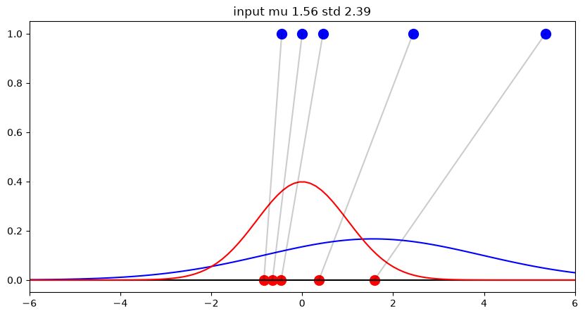
# Linear: activation statistics of forward and backward pass

g = torch.Generator().manual_seed(2147483647)

a = torch.randn((1000,1), requires_grad=True, generator=g)          # a.grad = b.T @ c.grad
b = torch.randn((1000,1000), requires_grad=True, generator=g)       # b.grad = c.grad @ a.T
c = b @ a
loss = torch.randn(1000, generator=g) @ c
a.retain_grad()
b.retain_grad()
c.retain_grad()
loss.backward()
print('a std:', a.std().item())
print('b std:', b.std().item())
print('c std:', c.std().item())
print('-----')
print('c grad std:', c.grad.std().item())
print('a grad std:', a.grad.std().item())
print('b grad std:', b.grad.std().item())
a std: 0.9875972270965576
b std: 1.0006722211837769
c std: 31.01241683959961
-----
c grad std: 0.9782556295394897
a grad std: 30.8818302154541
b grad std: 0.9666601419448853
# Linear + BatchNorm: activation statistics of forward and backward pass

g = torch.Generator().manual_seed(2147483647)

n = 1000
# linear layer ---
inp = torch.randn(n, requires_grad=True, generator=g)
w = torch.randn((n, n), requires_grad=True, generator=g) # / n**0.5
x = w @ inp
# bn layer ---
xmean = x.mean()
xvar = x.var()
out = (x - xmean) / torch.sqrt(xvar + 1e-5)
# ----
loss = out @ torch.randn(n, generator=g)
inp.retain_grad()
x.retain_grad()
w.retain_grad()
out.retain_grad()
loss.backward()

print('inp std: ', inp.std().item())
print('w std: ', w.std().item())
print('x std: ', x.std().item())
print('out std: ', out.std().item())
print('------')
print('out grad std: ', out.grad.std().item())
print('x grad std: ', x.grad.std().item())
print('w grad std: ', w.grad.std().item())
print('inp grad std: ', inp.grad.std().item())
inp std: 0.9875972270965576
w std: 1.0006722211837769
x std: 31.01241683959961
out std: 1.0
------
out grad std: 0.9782556295394897
x grad std: 0.031543977558612823
w grad std: 0.031169468536973
inp grad std: 0.9953053593635559