Embeddings and the MLP
Original study notes by Satish Bajagain, following Andrej Karpathy’s Zero to Hero. Comments, intermediate attempts and saved outputs are retained. Section titles are navigation additions.
Why learn an embedding?
# bigram model: good if we only have 1 character of previous context
# problem: predictions are not very good because we take only 1 character of context
# the problem with counts approach if we take more than 1 character for context: size of the table grows exponentially with the length of the context
# 1 char: 27 possibilities of context (27x27) entries, just 27 rows
# 2 char: 27x27 = 729 rows, 729x27 total entries
# 3 char: 27x27x27 = 19,683 possibilities of just context, 19,683x27 entries
# there'll be way too many rows, and way too few counts for each possibility
# thus, we're going to implement a MLP(multi-layer perceptron) model to predict the next character in the sequence
our approach follows the paper: Bengio et al. 2003
https://
# this paper wasn't the first to propose the use of MLP or neural networks to predict next char/token in a sequence
# very influential and often cited
# we're building a character level language model. In the paper, they have a vocabulary of 17,000 possible words
# and they built a word level language model
# but we're going to stick with the characters, and we'll take the same modeling approach they used# in the paper, they took each one of the 17,000 words and associated each word with a 30-dimensional feature vector
# i.e. embedding every single word into a 30 dimensional space
# initially, the words are spread out randomly, but then we tune the embedding of these words using backpropagation
# during the training of this neural network, these vectors are going to move around in space
# and the words that are synonyms or have very similar meanings end up in a very similar part of space
# conversely, words that mean very different things end up somewhere else in that 30 dimensional space
# in the paper, they are using a multi-layer neural network to predict the next word given the previous words
# to train the neural network, they are maximizing the log likelihood of the training data like we did# suppose our deployed model is trying to predict: A dog was running in a ..., but this example has never occured in training data
# though the model never saw this exact example, but maybe it has seen similar phrases like: The dog was running in a ...
# and maybe our network has learned that 'a' and 'the' are frequently interchangeable with one another
# so the model took the stored embedding for a and the which are nearby in space, then it can transfer knowledge to generalize
# similarly, the network could know that cats and dogs are animals and they co-occur in lots of similar context
# summary: model can transfer knowledge through the embedding space and then generalize to scenarios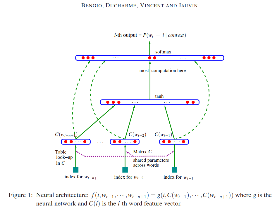
# in the above example, we are taking 3 previous words, then trying to predict the fourth word in the sequence
# we know that there are 17,000 possible words, so those 3 represent the index of the incoming word
# and that index for a single word, i.e. index for w(t-n+1), index for w(t-2) etc is an integer between 0 - 16,999
# There's a shared lookup table called C, this table is a matrix with dimensions: 17,000 x 30, and it is looked up over and over
# every index plucks out a row of that embedding matrix so that each index is converted to the 30-dimensional vector for that word
# After that, we see the input layer of 30 neurons for 3 words: total 90 neurons
# next is the hidden layer of this network
# the size of the hidden layer is a hyperparameter(meaning it is a design choice upto the designer of the neural net),
# i.e. the size of the hidden layer can be as large or as small as we like
# eg. size could be 100, and we will go over multiple choices of size, then we'll evaluate how they work
# eg. if we have 100 neurons in hidden layer, all of them will be fully connected to each of the 90 neurons
# then there is the tanh non-linearity
# then there is the output layer. Since there are 17,000 possible output words, the output layer has 17,000 neurons
# and all 100 neurons of hidden layer are also fully connected to all 17,000 neurons of the output layer
# thus, there are a lot of parameters there because there are a lot of words, making it most computation/expensive layer
# so, there are 17,000 logits(raw unscaled output generated by final layer of neural network before activation funcn like sigmoid or softmax) in output layer
# softmax: exponentiates every single logit, then everything is normalized to sum to 1
# finally, we get output as nice probability distribution for the next word in the sequence
# obviously during training, we have the identity of the label/(next word) in the sequence
# that word/label/index is used to pluck out the probability of that word, then we maximize the probability of that word w.r.t parameters of this neural net
# parameters: weights and biases of output layer, hidden layer, and the embedding look up table C
# all parameters are optimized using backpropagationConstructing the dataset
# for now: ignore that dashed arrows, they represent another variation of the neural net, not gonna explore nowimport torch
import torch.nn.functional as F
import matplotlib.pyplot as plt
%matplotlib inline# read all the words
words = open("names.txt", "r").read().splitlines()
print(words[:8])
print(len(words))['emma', 'olivia', 'ava', 'isabella', 'sophia', 'charlotte', 'mia', 'amelia']
32033
# build the vocabulary of characters and mappings to/from integers
chars = sorted(list(set(''.join(words))))
stoi = {s:i+1 for i,s in enumerate(chars)}
stoi['.'] = 0
print(stoi)
itos = {i:s for s,i in stoi.items()}
print(itos)
{'a': 1, 'b': 2, 'c': 3, 'd': 4, 'e': 5, 'f': 6, 'g': 7, 'h': 8, 'i': 9, 'j': 10, 'k': 11, 'l': 12, 'm': 13, 'n': 14, 'o': 15, 'p': 16, 'q': 17, 'r': 18, 's': 19, 't': 20, 'u': 21, 'v': 22, 'w': 23, 'x': 24, 'y': 25, 'z': 26, '.': 0}
{1: 'a', 2: 'b', 3: 'c', 4: 'd', 5: 'e', 6: 'f', 7: 'g', 8: 'h', 9: 'i', 10: 'j', 11: 'k', 12: 'l', 13: 'm', 14: 'n', 15: 'o', 16: 'p', 17: 'q', 18: 'r', 19: 's', 20: 't', 21: 'u', 22: 'v', 23: 'w', 24: 'x', 25: 'y', 26: 'z', 0: '.'}
# # example run for emma:
# context = [0,0,0]
# for ch in 'emma.':
#     ix = stoi[ch], ix = stoi[e] = 5
#     X.append(context), X.append([0,0,0])
#     Y.append(ix), Y.append(5)
#     display 000->5, i.e. ...->e
#     context = [0,0] + [5] = [0,0,5] #kinda like remove from left and add one to right cuz for next char, we need only 3 char

#     again
#     ix = stoi[ch], ix = stoi[m] = 13
#     X.append(context), X.append([0,0,5])
#     Y.append(ix), Y.append(13)
#     display 005->13, i.e. ..e->m
#     context = [0,5] + [13] = [0,5,13] #kinda like remove from left and add one to right cuz for next char, we need only 3 char

#     ....

#     similarly do until you reach last character .

#     ix = stoi[ch], ix = stoi[.] = 0
#     X.append(context), X.append([13,13,1])
#     Y.append(ix), Y.append(0)
#     display 13,13,1->0, i.e. mma->.
#     context = [13,1] + [0] = [13,1,0] #kinda like remove from left and add one to right cuz for next char, we need only 3 char
# we want to compile/build the dataset for this neural network
block_size = 3 # context length: how many characters to take as input to predict the single next character? #taking 3 cuz it's in paper though its for words
X, Y = [], [] #X: input to neural net, Y: labels/outputs for each example inside X
for w in words[:5]:
print(w)
context = [0] * block_size #start with padded context of just '0' tokens
for ch in w + '.':
ix = stoi[ch]#get the next character in sequence
X.append(context) #the current 3 characters
Y.append(ix) #the next character
print(''.join(itos[i] for i in context), '--->', itos[ix])
context = context[1:] + [ix] #crop and append, like a rolling window of context
X = torch.tensor(X)
Y = torch.tensor(Y)emma
... ---> e
..e ---> m
.em ---> m
emm ---> a
mma ---> .
olivia
... ---> o
..o ---> l
.ol ---> i
oli ---> v
liv ---> i
ivi ---> a
via ---> .
ava
... ---> a
..a ---> v
.av ---> a
ava ---> .
isabella
... ---> i
..i ---> s
.is ---> a
isa ---> b
sab ---> e
abe ---> l
bel ---> l
ell ---> a
lla ---> .
sophia
... ---> s
..s ---> o
.so ---> p
sop ---> h
oph ---> i
phi ---> a
hia ---> .
# the properties of dataset we built from the 5 words above
print(X.shape, X.dtype, Y.shape, Y.dtype)
# 32 examples from 5 words
torch.Size([32, 3]) torch.int64 torch.Size([32]) torch.int64
print(Y)
print(X)
tensor([ 5, 13, 13, 1, 0, 15, 12, 9, 22, 9, 1, 0, 1, 22, 1, 0, 9, 19,
1, 2, 5, 12, 12, 1, 0, 19, 15, 16, 8, 9, 1, 0])
tensor([[ 0, 0, 0],
[ 0, 0, 5],
[ 0, 5, 13],
[ 5, 13, 13],
[13, 13, 1],
[ 0, 0, 0],
[ 0, 0, 15],
[ 0, 15, 12],
[15, 12, 9],
[12, 9, 22],
[ 9, 22, 9],
[22, 9, 1],
[ 0, 0, 0],
[ 0, 0, 1],
[ 0, 1, 22],
[ 1, 22, 1],
[ 0, 0, 0],
[ 0, 0, 9],
[ 0, 9, 19],
[ 9, 19, 1],
[19, 1, 2],
[ 1, 2, 5],
[ 2, 5, 12],
[ 5, 12, 12],
[12, 12, 1],
[ 0, 0, 0],
[ 0, 0, 19],
[ 0, 19, 15],
[19, 15, 16],
[15, 16, 8],
[16, 8, 9],
[ 8, 9, 1]])
# let's write the neural network that takes the X's and predicts the Y'sEmbedding lookup
# First, let's build the embedding lookup table C
# we have 27 possible characters, and we're going to embed them in a lower dimensional space, eg. 2d space, later we'll increase it to check alternatives
# in paper, 17000 words embedded in 30-dimensional spaces
# lookup table initialized with random numbers has 27 rows and 2 columns. i.e. each char has 2 dimensional embeddings
C = torch.randn((27, 2))
Ctensor([[-0.4531, 1.8312],
[-1.1081, 1.2755],
[-0.4921, -1.5037],
[ 0.9516, -0.3177],
[-0.3224, -2.0600],
[ 1.2618, -0.6173],
[-1.4962, -0.9389],
[ 0.3770, 0.8204],
[ 0.0180, -0.2005],
[ 1.0692, 0.5852],
[-0.3504, -0.4033],
[-2.5449, 0.0481],
[ 0.9802, 0.3535],
[ 0.3050, 0.2734],
[ 1.5002, -1.2368],
[-0.6976, -0.4968],
[ 1.0344, 0.2092],
[-0.0621, -0.7390],
[ 1.0063, -1.2232],
[ 0.5172, -0.1634],
[-0.9044, -1.4194],
[ 0.0147, 1.4519],
[ 0.1422, 0.3577],
[-0.9049, -0.5961],
[-0.8813, 0.0410],
[ 0.0153, -0.3409],
[-0.5011, -0.2436]])# before embedding integer inputs in X using C, lets embed a single integer eg. 5 from X to understand how things work# one way to do it
C[5]tensor([ 1.2618, -0.6173])# another identical way we did previously is to use one-hot encoding to encode them
# F.one_hot(5, num_classes=27)
print(F.one_hot(torch.tensor(5), num_classes=27)) #27 vectors of 0s and 1s. 5th dimension vector = 1, all 26 other dimensions have values 0
print(F.one_hot(torch.tensor(5), num_classes=27).shape)
print(F.one_hot(torch.tensor(5), num_classes=27).dtype) #dtype of int64 means Long
# now, if we matrix multiply this one hot vector by C, we expect to pluck out the fifth row from C
# that's cuz all other 26 dimensions have values have 0 which mask out everything in C except for the fifth row
# F.one_hot(torch.tensor(5), num_classes=27) @ C
F.one_hot(torch.tensor(5), num_classes=27).float() @ Ctensor([0, 0, 0, 0, 0, 1, 0, 0, 0, 0, 0, 0, 0, 0, 0, 0, 0, 0, 0, 0, 0, 0, 0, 0,
0, 0, 0])
torch.Size([27])
torch.int64
tensor([ 1.2618, -0.6173])# Interpreting the embedding of the integer
# think of it as: integer indexing upto the lookup table C as C[i]
# or equivalently think of it as: first layer of neural net whose weight matrix is C, we're encoding integers into one-hot and feeding it into neural net
# and the first layer embeds them# but we're just going to use C[5] instead of one hot F.one_hot(torch.tensor(5), num_classes=27).float() @ C
# because just indexing C[5] is faster# embeding a single integer is easy
# but how do we embed all 32x3 integers stored in X
# luckily, pytorch indexing is powerful and flexible
X.shapetorch.Size([32, 3])# index using lists, tensors
C[[5,6,7]]
C[torch.tensor([5,6,7])]
C[torch.tensor([5,6,7, 7, 7, 7, 7, 7])] #indexing with one dimensional tensor of integerstensor([[ 1.2618, -0.6173],
[-1.4962, -0.9389],
[ 0.3770, 0.8204],
[ 0.3770, 0.8204],
[ 0.3770, 0.8204],
[ 0.3770, 0.8204],
[ 0.3770, 0.8204],
[ 0.3770, 0.8204]])Xtensor([[ 0, 0, 0],
[ 0, 0, 5],
[ 0, 5, 13],
[ 5, 13, 13],
[13, 13, 1],
[ 0, 0, 0],
[ 0, 0, 15],
[ 0, 15, 12],
[15, 12, 9],
[12, 9, 22],
[ 9, 22, 9],
[22, 9, 1],
[ 0, 0, 0],
[ 0, 0, 1],
[ 0, 1, 22],
[ 1, 22, 1],
[ 0, 0, 0],
[ 0, 0, 9],
[ 0, 9, 19],
[ 9, 19, 1],
[19, 1, 2],
[ 1, 2, 5],
[ 2, 5, 12],
[ 5, 12, 12],
[12, 12, 1],
[ 0, 0, 0],
[ 0, 0, 19],
[ 0, 19, 15],
[19, 15, 16],
[15, 16, 8],
[16, 8, 9],
[ 8, 9, 1]])Ctensor([[-0.4531, 1.8312],
[-1.1081, 1.2755],
[-0.4921, -1.5037],
[ 0.9516, -0.3177],
[-0.3224, -2.0600],
[ 1.2618, -0.6173],
[-1.4962, -0.9389],
[ 0.3770, 0.8204],
[ 0.0180, -0.2005],
[ 1.0692, 0.5852],
[-0.3504, -0.4033],
[-2.5449, 0.0481],
[ 0.9802, 0.3535],
[ 0.3050, 0.2734],
[ 1.5002, -1.2368],
[-0.6976, -0.4968],
[ 1.0344, 0.2092],
[-0.0621, -0.7390],
[ 1.0063, -1.2232],
[ 0.5172, -0.1634],
[-0.9044, -1.4194],
[ 0.0147, 1.4519],
[ 0.1422, 0.3577],
[-0.9049, -0.5961],
[-0.8813, 0.0410],
[ 0.0153, -0.3409],
[-0.5011, -0.2436]])C[X] #indexing with multi dimensional tensor of integerstensor([[[-0.4531, 1.8312],
[-0.4531, 1.8312],
[-0.4531, 1.8312]],
[[-0.4531, 1.8312],
[-0.4531, 1.8312],
[ 1.2618, -0.6173]],
[[-0.4531, 1.8312],
[ 1.2618, -0.6173],
[ 0.3050, 0.2734]],
[[ 1.2618, -0.6173],
[ 0.3050, 0.2734],
[ 0.3050, 0.2734]],
[[ 0.3050, 0.2734],
[ 0.3050, 0.2734],
[-1.1081, 1.2755]],
[[-0.4531, 1.8312],
[-0.4531, 1.8312],
[-0.4531, 1.8312]],
[[-0.4531, 1.8312],
[-0.4531, 1.8312],
[-0.6976, -0.4968]],
[[-0.4531, 1.8312],
[-0.6976, -0.4968],
[ 0.9802, 0.3535]],
[[-0.6976, -0.4968],
[ 0.9802, 0.3535],
[ 1.0692, 0.5852]],
[[ 0.9802, 0.3535],
[ 1.0692, 0.5852],
[ 0.1422, 0.3577]],
[[ 1.0692, 0.5852],
[ 0.1422, 0.3577],
[ 1.0692, 0.5852]],
[[ 0.1422, 0.3577],
[ 1.0692, 0.5852],
[-1.1081, 1.2755]],
[[-0.4531, 1.8312],
[-0.4531, 1.8312],
[-0.4531, 1.8312]],
[[-0.4531, 1.8312],
[-0.4531, 1.8312],
[-1.1081, 1.2755]],
[[-0.4531, 1.8312],
[-1.1081, 1.2755],
[ 0.1422, 0.3577]],
[[-1.1081, 1.2755],
[ 0.1422, 0.3577],
[-1.1081, 1.2755]],
[[-0.4531, 1.8312],
[-0.4531, 1.8312],
[-0.4531, 1.8312]],
[[-0.4531, 1.8312],
[-0.4531, 1.8312],
[ 1.0692, 0.5852]],
[[-0.4531, 1.8312],
[ 1.0692, 0.5852],
[ 0.5172, -0.1634]],
[[ 1.0692, 0.5852],
[ 0.5172, -0.1634],
[-1.1081, 1.2755]],
[[ 0.5172, -0.1634],
[-1.1081, 1.2755],
[-0.4921, -1.5037]],
[[-1.1081, 1.2755],
[-0.4921, -1.5037],
[ 1.2618, -0.6173]],
[[-0.4921, -1.5037],
[ 1.2618, -0.6173],
[ 0.9802, 0.3535]],
[[ 1.2618, -0.6173],
[ 0.9802, 0.3535],
[ 0.9802, 0.3535]],
[[ 0.9802, 0.3535],
[ 0.9802, 0.3535],
[-1.1081, 1.2755]],
[[-0.4531, 1.8312],
[-0.4531, 1.8312],
[-0.4531, 1.8312]],
[[-0.4531, 1.8312],
[-0.4531, 1.8312],
[ 0.5172, -0.1634]],
[[-0.4531, 1.8312],
[ 0.5172, -0.1634],
[-0.6976, -0.4968]],
[[ 0.5172, -0.1634],
[-0.6976, -0.4968],
[ 1.0344, 0.2092]],
[[-0.6976, -0.4968],
[ 1.0344, 0.2092],
[ 0.0180, -0.2005]],
[[ 1.0344, 0.2092],
[ 0.0180, -0.2005],
[ 1.0692, 0.5852]],
[[ 0.0180, -0.2005],
[ 1.0692, 0.5852],
[-1.1081, 1.2755]]])print(X.shape)
print(C.shape)
print(C[X].shape)
# for every one of the 32x3 input (eg. ..., ..e, .em, emm, mma, etc), we retrieved the embedding vector (dimension 2)torch.Size([32, 3])
torch.Size([27, 2])
torch.Size([32, 3, 2])
# eg. for input
print(X[3])
print(C[X][3])
print(X[3, 2])
print(C[X][3,2])
tensor([ 5, 13, 13])
tensor([[ 1.2618, -0.6173],
[ 0.3050, 0.2734],
[ 0.3050, 0.2734]])
tensor(13)
tensor([0.3050, 0.2734])
C[13]tensor([0.3050, 0.2734])# long story short: pytorch indexing is awesome, and for our embedding we can do simply C[X] for all integers in Xemb = C[X]
emb.shapetorch.Size([32, 3, 2])# now, we'll construct the hidden layer
# no of inputs to each neuron in hidden layer will be 3x2 = 6 because we have 2-dimensional embeddings and we have three of them
# and number of neurons is upto us eg. 100
# initialize weights and biases initially randomly
W1= torch.randn((6, 100))
b1 = torch.randn(100)# now, normally we'd do emb @ W1 + b1
# but the problem is that the embeddings are stacked up in the dimensions of the input tensor
# i.e. its emb.shape is 32x3x2 but W1's shape is 6x100 and it isn't matrix multiplicable
# so we need to transform 32x3x2 to 32x6, how to concatenate? look at pytorch documentationTensor shapes and views
# look at the figure above, we just want to retreive the 3 parts and concatenate them
print(emb.shape)
print(emb[:].shape)
print(emb[:, 0].shape) #plucks the 32x2 embeddings of just the first context letter
print(emb[:, 1].shape) #plucks the 32x2 embeddings of just the second context letter
print(emb[:, 2].shape) #plucks the 32x2 embeddings of just the third context letter
# print(torch.cat([emb[:, 0], emb[:, 1], emb[:, 2]]).shape) #this concatenates across dimension 0, but we should do along dimension 1
torch.cat([emb[:, 0], emb[:, 1], emb[:, 2]], 1).shape
# this is less efficient as it will create a whole new tensor with whole new storage during concatenation

# but this code won't generalize if we later want to change the block size
# there is torch.unbind: removes a tensor dimension, returns a tuple of slices along a given dimension, already without it.
torch.Size([32, 3, 2])
torch.Size([32, 3, 2])
torch.Size([32, 2])
torch.Size([32, 2])
torch.Size([32, 2])
torch.Size([32, 6])# torch.unbind(emb, 1) (the 1 stands for dimension 1 i.e. 3 in 32x3x2) gives a list equivalent to [emb[:, 0], emb[:, 1], emb[:, 2]
# print(torch.unbind(emb, 1))
len(torch.unbind(emb, 1))3# print([emb[:, 0]], [emb[:, 1]], [emb[:, 2]])torch.cat(torch.unbind(emb, 1), 1).shapetorch.Size([32, 6])# but there's an even better way to do it
a = torch.arange(18)
print(a)
a.shapetensor([ 0, 1, 2, 3, 4, 5, 6, 7, 8, 9, 10, 11, 12, 13, 14, 15, 16, 17])
torch.Size([18])# we can re-represent it as different sized n-dimensional tensors by calling a view
# we can convert a single vector of length 18 to a 2x9 tensor or whatever as long as the product of numbers result in the same
print(a.view(2,9))
# print(a.view(9, 2))
# print(a.view(3,6))
print(a.view(3,3,2))tensor([[ 0, 1, 2, 3, 4, 5, 6, 7, 8],
[ 9, 10, 11, 12, 13, 14, 15, 16, 17]])
tensor([[[ 0, 1],
[ 2, 3],
[ 4, 5]],
[[ 6, 7],
[ 8, 9],
[10, 11]],
[[12, 13],
[14, 15],
[16, 17]]])
# this view operation is extremely efficient cuz in each tensor there's something called an underlying storage
# and the storage is just the numbers always as a 1-dimensional vector in memory
# when view is called, no memory is being changed, copied, created
# storage is identical, but when view is called, some of the internal attributes of the view of this tensor are being manipulated
# storage offset, strides, shapes are manipulated so that this one dimensional sequence of bytes is seen as different n-dimensional arrays
print(emb.shape)
# but lol, we can just do view
print(emb.view(32,6).shape)
# verify the result
torch.cat(torch.unbind(emb, 1), 1) == emb.view(32,6)torch.Size([32, 3, 2])
torch.Size([32, 6])
tensor([[True, True, True, True, True, True],
        [True, True, True, True, True, True],
        [True, True, True, True, True, True],
        [True, True, True, True, True, True],
        [True, True, True, True, True, True],
        [True, True, True, True, True, True],
        [True, True, True, True, True, True],
        [True, True, True, True, True, True],
        [True, True, True, True, True, True],
        [True, True, True, True, True, True],
        [True, True, True, True, True, True],
        [True, True, True, True, True, True],
        [True, True, True, True, True, True],
        [True, True, True, True, True, True],
        [True, True, True, True, True, True],
        [True, True, True, True, True, True],
        [True, True, True, True, True, True],
        [True, True, True, True, True, True],
        [True, True, True, True, True, True],
        [True, True, True, True, True, True],
        [True, True, True, True, True, True],
        [True, True, True, True, True, True],
        [True, True, True, True, True, True],
        [True, True, True, True, True, True],
        [True, True, True, True, True, True],
        [True, True, True, True, True, True],
        [True, True, True, True, True, True],
        [True, True, True, True, True, True],
        [True, True, True, True, True, True],
        [True, True, True, True, True, True],
        [True, True, True, True, True, True],
        [True, True, True, True, True, True]])
# so, we can make the matrix multiplication work for hidden layer
h = emb.view(32,6) @ W1 + b1
print(h.shape)
print(h)torch.Size([32, 100])
tensor([[ 2.1610, -0.2779, -3.3302, ..., -5.3586, -2.5805, 7.6029],
[-1.7104, -2.9558, 2.7157, ..., -3.5984, -2.2396, 1.5187],
[-0.1398, -1.9331, -1.5896, ..., 0.6374, -4.6067, -2.8069],
...,
[ 2.7360, -0.9866, -1.5149, ..., 1.1118, -2.1364, -1.9223],
[ 0.9865, -1.4296, 2.7832, ..., -1.4004, -1.9962, 0.6385],
[ 4.3424, 1.3410, -3.2238, ..., -1.0142, -2.9415, 1.9439]])
# better not to hardcode the numbers
# h = emb.view(emb.shape[0],6) @ W1 + b1
# or we can do just -1: then pytorch will itself infer what it should be, pytorch will find the 32 itself
h = emb.view(-1,6) @ W1 + b1
print(h)
print(h.shape)
tensor([[ 2.1610, -0.2779, -3.3302, ..., -5.3586, -2.5805, 7.6029],
[-1.7104, -2.9558, 2.7157, ..., -3.5984, -2.2396, 1.5187],
[-0.1398, -1.9331, -1.5896, ..., 0.6374, -4.6067, -2.8069],
...,
[ 2.7360, -0.9866, -1.5149, ..., 1.1118, -2.1364, -1.9223],
[ 0.9865, -1.4296, 2.7832, ..., -1.4004, -1.9962, 0.6385],
[ 4.3424, 1.3410, -3.2238, ..., -1.0142, -2.9415, 1.9439]])
torch.Size([32, 100])
# also find tanh
h = torch.tanh(emb.view(-1,6) @ W1 + b1)
# the nums are now between -1 and 1

print(h.shape)
print(h)
torch.Size([32, 100])
tensor([[ 0.9738, -0.2709, -0.9974, ..., -1.0000, -0.9886, 1.0000],
[-0.9367, -0.9946, 0.9913, ..., -0.9985, -0.9776, 0.9085],
[-0.1389, -0.9590, -0.9201, ..., 0.5631, -0.9998, -0.9927],
...,
[ 0.9916, -0.7559, -0.9078, ..., 0.8047, -0.9725, -0.9581],
[ 0.7559, -0.8916, 0.9924, ..., -0.8854, -0.9638, 0.5639],
[ 0.9997, 0.8719, -0.9968, ..., -0.7675, -0.9944, 0.9598]])
# also here: emb.view(-1,6) @ W1 + b1, we want to make sure our broadcasting does what we like
print((emb.view(-1,6) @ W1).shape)
print(b1.shape)
torch.Size([32, 100])
torch.Size([100])
# 32 x 100
 # 1 x 100 #will create fake count 1, and copy itself vertically to every one of the 32 rows and do element wise addition
# to create the final layer
W2 = torch.randn((100, 27))
b2 = torch.randn(27)logits = h @ W2 + b2
logits.shapetorch.Size([32, 27])logitstensor([[-1.2847e+01, 1.0026e+01, 1.9691e+00, 7.6149e+00, -5.1461e+00,
-2.3212e+00, -3.6223e+00, 1.1467e+01, 1.3246e+01, 3.7298e+00,
3.7574e+00, 7.8842e+00, 4.0562e+00, 4.7126e+00, 1.0140e+01,
3.4464e-01, -1.9649e+00, 6.1454e+00, -1.3081e+01, 9.9285e+00,
2.4812e-01, -1.6957e+00, 3.3765e-01, -1.3276e+01, 7.4120e+00,
1.0150e+01, -4.4334e+00],
[-1.3620e+01, -1.3657e+00, -1.1359e+00, -6.8896e+00, -2.0300e+00,
-9.7428e-01, -1.7288e+00, 1.5028e+01, 1.3833e+01, -1.9324e+00,
-3.3925e+00, -8.6331e+00, 1.3026e+01, 4.9972e+00, 1.6434e+01,
6.0610e+00, -5.4358e+00, 1.9138e+00, -1.0739e+01, -6.5129e+00,
-2.8064e+00, -4.1982e+00, -1.4904e+00, -9.6555e+00, -4.0858e+00,
6.9395e+00, -8.2195e+00],
[-1.2651e+01, -5.4040e+00, 5.4297e-02, -1.5112e+01, -1.0523e+00,
2.3478e+00, -2.4818e+00, 1.0362e+00, 7.0741e+00, -5.4762e+00,
1.0416e+01, -3.7080e+00, 6.9962e+00, 3.1877e+00, 3.4941e+00,
1.2851e+01, 1.9367e+00, 2.0149e+00, 2.8327e+00, 5.9749e+00,
2.4387e+00, -4.3836e+00, -5.0668e+00, -1.1957e+01, -5.9885e-01,
-6.2009e-01, 3.8546e+00],
[ 4.1554e+00, 3.5724e+00, 1.4581e+00, 1.0070e+01, 6.4821e-01,
-1.2471e+01, -2.7371e+00, 2.2192e+01, 6.4888e-01, 1.2743e+01,
3.4793e+00, -5.7745e+00, 6.3882e+00, 1.1913e+00, -7.9579e+00,
-1.5995e+01, -1.3742e+01, -1.1918e+01, -1.0744e-01, -9.2285e+00,
-1.0003e+01, -1.0554e+00, 7.1328e+00, 5.6721e+00, 8.2260e+00,
-1.0271e+01, -1.3062e-01],
[-4.6347e-01, 8.8664e+00, 3.1043e+00, 1.4674e+01, -4.2495e+00,
-6.0670e+00, 1.6563e+00, 8.9288e+00, 6.2872e+00, 1.1663e+01,
1.7686e+01, 1.2456e+01, 3.4402e+00, -2.7428e+00, -1.2264e+01,
-5.5284e+00, -5.0609e-01, -1.1759e+00, -3.8059e-01, 4.0245e+00,
-2.5362e-01, -1.4547e-01, 5.8460e+00, -1.2252e+01, 1.1325e+01,
-1.2265e+01, 2.3568e-01],
[-1.2847e+01, 1.0026e+01, 1.9691e+00, 7.6149e+00, -5.1461e+00,
-2.3212e+00, -3.6223e+00, 1.1467e+01, 1.3246e+01, 3.7298e+00,
3.7574e+00, 7.8842e+00, 4.0562e+00, 4.7126e+00, 1.0140e+01,
3.4464e-01, -1.9649e+00, 6.1454e+00, -1.3081e+01, 9.9285e+00,
2.4812e-01, -1.6957e+00, 3.3765e-01, -1.3276e+01, 7.4120e+00,
1.0150e+01, -4.4334e+00],
[-1.4972e+01, 9.2175e+00, 2.8487e+00, 3.2509e+00, 6.8963e+00,
-7.5028e-01, 6.9758e+00, 7.3064e+00, 1.6497e+01, 2.2311e+00,
-2.3180e+00, 1.5126e+00, 4.9568e+00, 4.9983e+00, 1.1253e+01,
2.3264e+00, 6.4658e+00, 1.1565e+00, -1.0150e+01, 4.1034e+00,
2.9045e+00, -2.4206e+00, -2.8317e+00, -2.2917e+01, 8.5607e+00,
-1.4634e+00, -8.0242e+00],
[-4.0764e+00, -6.5541e+00, 1.1152e+01, -9.1724e+00, 2.4697e+00,
1.1678e+00, 1.8115e+00, 2.0279e+00, 1.9988e+00, 5.4031e+00,
8.9813e+00, -3.9090e+00, -6.4136e+00, 1.8600e+00, 8.6545e+00,
4.6729e+00, 4.9382e+00, -1.3235e+00, 6.8951e+00, -2.1259e+00,
9.8535e+00, -3.6721e+00, -1.2282e+00, -1.5148e+01, -1.0340e+01,
5.6368e-01, -5.4027e+00],
[-2.7329e+00, 2.7130e-01, -4.3298e+00, -1.1150e+01, -1.5816e+01,
1.7348e+00, -9.4273e+00, 8.1684e+00, 3.3047e+00, -1.3047e+01,
6.8526e+00, -5.0262e+00, 1.3803e+01, 1.5517e+01, 1.6600e+00,
9.4302e+00, -7.7696e+00, 2.5172e+00, -2.7048e+00, -4.1037e+00,
-4.9364e+00, 2.4009e+00, -3.1375e+00, -3.3835e+00, -1.3874e+01,
5.5346e+00, 4.2792e+00],
[ 7.7615e-01, 8.2894e+00, -1.0955e-01, 6.1125e+00, 6.3437e+00,
-1.3885e+01, -8.2639e+00, 1.9669e+01, 1.0263e+01, 1.4868e+00,
3.9244e+00, -6.4716e+00, 1.8685e+01, -3.5847e-01, -1.1571e+01,
-1.0808e+01, -1.1849e+01, -3.4079e+00, -6.4316e+00, -3.1043e+00,
-4.3971e+00, -1.6824e+00, 7.9437e+00, -6.8012e-01, 1.0788e+01,
-8.2015e+00, -2.4026e+00],
[-3.9857e+00, 1.6324e+00, -3.9148e+00, 4.1553e+00, 5.5246e+00,
-1.3492e+01, -2.3744e+00, 2.3716e+01, 6.4340e+00, 8.5696e+00,
2.5836e+00, -1.2697e+01, 1.5262e+01, -7.3406e+00, 1.8163e+00,
-1.7313e+01, -1.5364e+01, -9.7115e+00, -2.2693e+00, -5.5836e+00,
7.7385e-01, -3.8181e-01, 4.9681e+00, 5.8310e+00, 4.1233e+00,
-4.9692e-01, -2.3542e+00],
[-4.8402e+00, 8.1008e+00, 6.0202e-01, 1.3071e+01, -2.8462e+00,
-4.4160e+00, -6.9501e-01, 6.4765e+00, 7.3834e+00, 6.5988e+00,
1.4318e+01, 8.6077e+00, 9.6439e+00, -2.2269e-02, -1.2773e+01,
1.5920e+00, -3.1530e+00, 1.2984e+00, -2.0358e+00, 3.9828e+00,
-1.8072e-01, 2.7062e-01, 2.6784e+00, -1.2756e+01, 1.3030e+01,
-9.3931e+00, 3.5574e+00],
[-1.2847e+01, 1.0026e+01, 1.9691e+00, 7.6149e+00, -5.1461e+00,
-2.3212e+00, -3.6223e+00, 1.1467e+01, 1.3246e+01, 3.7298e+00,
3.7574e+00, 7.8842e+00, 4.0562e+00, 4.7126e+00, 1.0140e+01,
3.4464e-01, -1.9649e+00, 6.1454e+00, -1.3081e+01, 9.9285e+00,
2.4812e-01, -1.6957e+00, 3.3765e-01, -1.3276e+01, 7.4120e+00,
1.0150e+01, -4.4334e+00],
[-1.5092e+01, 1.2038e+01, 1.2964e+00, 1.2389e+01, -1.4539e+00,
-7.9082e-03, -3.3734e-01, 7.4867e+00, 1.3930e+01, 5.1877e+00,
2.2226e+00, 9.2452e+00, 4.0382e+00, 1.7279e+00, 8.7634e+00,
7.1712e-01, 8.4681e-01, 4.7628e+00, -1.1895e+01, 1.2348e+01,
4.5150e+00, 4.2484e-01, 9.7787e-01, -1.7187e+01, 1.2356e+01,
6.2102e+00, -3.7324e+00],
[-8.9008e+00, 4.4080e+00, 4.4318e+00, 2.2540e+00, -1.2675e+00,
-3.3090e-01, 1.6452e+00, 1.3611e+01, 1.2269e+01, 7.2365e+00,
4.2343e+00, -1.7912e+00, 1.6684e+00, 1.9667e+00, 1.5414e+01,
6.3291e-01, 2.6747e+00, -3.9901e-01, -7.2592e+00, 2.7040e+00,
3.5770e+00, -4.9301e+00, -2.7507e+00, -1.4508e+01, -2.8077e-01,
4.7733e+00, -4.7988e+00],
[-1.2758e+01, 2.2382e+00, 2.4066e+00, 1.1060e+01, -4.9990e+00,
5.2156e+00, -4.4426e+00, 1.6792e+00, 1.2021e+01, -2.1027e-03,
9.1578e+00, 1.3067e+01, -2.2217e-01, 8.2486e+00, 2.5665e+00,
9.6489e+00, 2.8399e+00, -2.7094e-02, -2.3976e-01, 1.1500e+01,
7.1971e+00, 2.3944e+00, -6.4115e+00, -2.0295e+01, 1.1305e+01,
8.0893e+00, 3.1517e+00],
[-1.2847e+01, 1.0026e+01, 1.9691e+00, 7.6149e+00, -5.1461e+00,
-2.3212e+00, -3.6223e+00, 1.1467e+01, 1.3246e+01, 3.7298e+00,
3.7574e+00, 7.8842e+00, 4.0562e+00, 4.7126e+00, 1.0140e+01,
3.4464e-01, -1.9649e+00, 6.1454e+00, -1.3081e+01, 9.9285e+00,
2.4812e-01, -1.6957e+00, 3.3765e-01, -1.3276e+01, 7.4120e+00,
1.0150e+01, -4.4334e+00],
[-1.2652e+01, 3.9511e+00, -5.1430e+00, -7.1475e+00, -4.9583e+00,
-2.9617e+00, -5.2105e+00, 1.7187e+01, 1.6116e+01, 3.8775e-02,
2.7555e+00, -8.6077e+00, 8.3470e+00, 3.2345e+00, 1.7911e+01,
6.4534e+00, -3.9748e+00, 3.1233e+00, -1.2611e+01, -1.8812e+00,
-1.3201e+00, -1.4820e+00, 1.1757e+00, -1.2515e+01, -6.0736e+00,
1.0172e+01, -3.5326e+00],
[-1.2935e+01, 1.3737e+00, -4.1921e+00, -1.5166e+01, 1.3288e+00,
-5.1022e-01, -7.9726e+00, 3.9243e+00, 1.7807e+01, -9.0930e+00,
-2.0359e-02, 1.7367e+00, 9.6494e+00, 8.2971e+00, 1.0358e+01,
1.1226e+01, -3.9203e+00, 3.3498e-01, -8.3871e+00, -5.4843e-01,
5.9150e-01, -3.5016e+00, -1.0876e+00, -1.2555e+01, -5.0847e-01,
5.8621e+00, -4.8639e+00],
[ 1.0161e-01, 6.6007e+00, 9.8069e+00, 1.4821e+01, 1.2236e+00,
-9.6462e+00, 1.4787e+00, 1.3373e+01, 1.8725e+00, 1.3183e+01,
1.3480e+01, 1.0190e+01, 2.6613e+00, -8.3635e+00, -1.5940e+01,
-1.2331e+01, -1.6309e-01, -5.7153e+00, 1.5361e+00, -1.9461e-01,
3.6777e-01, -3.5551e+00, 1.2374e+01, -9.9420e+00, 1.2890e+01,
-1.6508e+01, -1.3554e-01],
[ 4.9738e+00, 6.1426e+00, 1.6289e+00, 7.1519e+00, 3.8647e+00,
-9.0524e+00, 7.2859e+00, 1.1297e+01, 5.9817e+00, 1.1867e+01,
-1.0214e+01, -9.1833e+00, 2.1666e+00, 1.6104e+00, 3.1599e+00,
-7.6476e+00, 2.3874e+00, -1.2645e+00, -3.2223e+00, -4.3432e+00,
-7.7958e+00, 9.9867e-01, -1.0731e+00, -8.1652e+00, 9.0796e+00,
-3.2359e+00, -1.0371e+01],
[ 1.8241e+00, -1.3868e+01, 1.4020e+01, -1.5965e+01, 1.0701e+00,
5.4444e+00, 4.2917e-01, -5.7515e-01, -2.8100e+00, -2.8709e+00,
7.1266e+00, -3.1511e+00, -8.0580e+00, 6.6658e+00, 7.0846e+00,
1.2730e+01, 8.7670e+00, -4.1678e-01, 1.5756e+01, 5.1726e+00,
1.0376e+00, -1.0713e+01, -6.8073e+00, -8.5149e+00, -1.7745e+01,
3.2241e+00, 5.2405e+00],
[ 5.5199e+00, -3.9504e+00, -1.5806e+00, -1.0202e+01, -1.0506e+01,
-6.6235e+00, -8.4520e+00, 7.3821e+00, -3.0211e+00, -8.3313e+00,
6.3300e+00, -5.7338e+00, 3.7462e+00, 5.2676e+00, -1.3236e+01,
8.2941e+00, -8.4889e+00, -2.9293e+00, 8.5216e+00, 3.4076e+00,
-5.2235e+00, 3.5835e+00, -4.8874e+00, 6.8935e+00, -1.5550e+01,
2.7070e+00, 1.1500e+01],
[ 5.0944e+00, 3.0900e+00, -1.1976e+00, 3.1253e+00, -2.3990e+00,
-1.3011e+01, -6.3930e+00, 2.9700e+01, 1.0290e+00, 5.6567e+00,
-6.5736e-01, -9.7826e+00, 1.2273e+01, 3.3388e+00, -6.6630e+00,
-8.9630e+00, -1.7900e+01, -7.0917e+00, -3.1173e+00, -7.7430e+00,
-1.3580e+01, -3.3932e+00, 8.1745e+00, 1.0373e+01, 5.2421e+00,
-6.4964e+00, 3.5419e+00],
[ 2.0159e+00, 8.8060e+00, 4.0063e+00, 1.6669e+01, 3.0144e+00,
-1.1584e+01, -2.5490e+00, 9.8416e+00, 3.8918e+00, 1.2022e+01,
1.4006e+01, 9.2304e+00, 6.8386e+00, -6.7302e+00, -1.7520e+01,
-1.3354e+01, -4.7339e+00, -3.9415e+00, -1.6684e+00, -1.3394e+00,
-8.2958e-01, -6.9961e-02, 1.1717e+01, -1.0342e+01, 1.2262e+01,
-1.4000e+01, -4.6814e-01],
[-1.2847e+01, 1.0026e+01, 1.9691e+00, 7.6149e+00, -5.1461e+00,
-2.3212e+00, -3.6223e+00, 1.1467e+01, 1.3246e+01, 3.7298e+00,
3.7574e+00, 7.8842e+00, 4.0562e+00, 4.7126e+00, 1.0140e+01,
3.4464e-01, -1.9649e+00, 6.1454e+00, -1.3081e+01, 9.9285e+00,
2.4812e-01, -1.6957e+00, 3.3765e-01, -1.3276e+01, 7.4120e+00,
1.0150e+01, -4.4334e+00],
[-1.1418e+01, 2.7066e+00, -1.4704e+00, -7.8454e+00, -8.6202e-02,
-4.1806e-01, -2.5269e+00, 1.3407e+01, 1.8095e+01, -3.5984e+00,
-2.2550e-01, -5.4091e+00, 1.0011e+01, 6.0928e+00, 1.4850e+01,
2.9913e+00, -3.8415e+00, 1.4412e+00, -1.4033e+01, -2.9747e+00,
-2.3229e+00, -4.6124e+00, -1.2355e+00, -1.4682e+01, -1.2088e+00,
5.8062e+00, -7.4217e+00],
[-1.1778e+01, -2.3414e+00, 1.0509e+01, -9.9139e+00, 6.6271e+00,
-1.6409e+00, 6.7909e+00, 2.0028e+00, 1.8457e+01, -1.3524e+00,
1.1436e+00, 3.7894e+00, 6.4140e-02, 5.1844e+00, 3.7040e+00,
1.7578e+01, 9.4013e+00, -5.1125e+00, -1.0358e+00, 8.3479e+00,
8.6086e+00, -1.5670e+00, -4.6422e+00, -2.3278e+01, 4.2686e+00,
4.1056e+00, -4.2517e+00],
[ 6.4243e+00, -8.4955e+00, 5.3884e+00, -6.0094e+00, -4.5648e+00,
-3.1719e+00, 3.5821e+00, 1.3634e+01, -1.1372e+01, 6.0907e+00,
1.0763e+01, -1.2052e+01, -2.0525e+00, -7.5481e-01, 2.9314e+00,
-8.6747e+00, -7.1567e+00, -1.1080e+01, 1.6390e+01, -4.4098e+00,
2.2564e-01, -2.7739e+00, -2.1183e+00, 3.0867e+00, -8.2940e+00,
-5.9006e+00, 9.2862e-02],
[-3.9568e+00, 6.0253e-02, 5.6556e-01, -1.1565e+01, -2.2095e+01,
-4.0137e+00, -5.3736e+00, 7.2948e+00, 7.3401e+00, -1.4248e+01,
3.2722e+00, 2.3503e+00, 2.8692e-01, 1.2277e+01, -3.7488e+00,
1.7510e+01, 4.4332e-01, 2.8671e+00, 4.8864e+00, -1.2424e+00,
-4.7542e+00, -7.8932e-01, -5.7761e+00, -8.0429e+00, -9.0605e+00,
4.4295e+00, 6.7721e+00],
[-1.0693e+00, -2.4629e+00, -9.9557e-01, 1.4367e+00, 2.0410e+00,
-1.0033e+01, -9.7149e-01, 2.2781e+01, -8.4663e-01, 5.3276e+00,
1.0090e+01, -1.1237e+01, 9.4750e+00, -4.6984e+00, -2.7679e-01,
-1.5068e+01, -1.4819e+01, -1.1257e+01, 4.3066e+00, -7.7518e+00,
-2.4472e+00, -2.4119e+00, 6.2488e+00, 8.4056e+00, -5.3557e-01,
-3.9582e+00, -3.1668e+00],
[ 2.3242e+00, 2.2812e+00, 1.2239e+00, 1.2120e+01, -3.4779e+00,
-4.4262e+00, -1.9541e+00, 7.3218e+00, 5.6649e+00, 5.6822e+00,
1.3200e+01, 9.6747e+00, 8.9556e+00, -2.0783e+00, -1.2010e+01,
3.7965e+00, -4.3494e+00, 1.7220e+00, -2.9707e+00, 1.4447e+00,
3.6450e-01, 1.3994e+00, -9.0826e-01, -1.3983e+01, 8.5225e+00,
-8.7139e+00, 5.7461e+00]])counts = logits.exp()
probs = counts / counts.sum(1, keepdims=True)
probs.shapetorch.Size([32, 27])probs[0].sum()tensor(1.)probstensor([[3.4559e-12, 2.9661e-02, 9.3958e-06, 2.6598e-03, 7.6356e-09, 1.2873e-07,
3.5043e-08, 1.2520e-01, 7.4220e-01, 5.4649e-05, 5.6180e-05, 3.4819e-03,
7.5743e-05, 1.4603e-04, 3.3219e-02, 1.8511e-06, 1.8382e-07, 6.1188e-04,
2.7327e-12, 2.6893e-02, 1.6808e-06, 2.4062e-07, 1.8382e-06, 2.2499e-12,
2.1714e-03, 3.3549e-02, 1.5573e-08],
[6.5544e-14, 1.3756e-08, 1.7311e-08, 5.4896e-11, 7.0799e-09, 2.0348e-08,
9.5685e-09, 1.8127e-01, 5.4880e-02, 7.8058e-09, 1.8125e-09, 9.6014e-12,
2.4487e-02, 7.9781e-06, 7.3928e-01, 2.3114e-05, 2.3491e-10, 3.6540e-07,
1.1692e-12, 8.0005e-11, 3.2572e-09, 8.0980e-10, 1.2144e-08, 3.4540e-12,
9.0612e-10, 5.5643e-05, 1.4519e-11],
[7.6808e-12, 1.0779e-08, 2.5298e-06, 6.5512e-13, 8.3656e-07, 2.5068e-05,
2.0029e-07, 6.7535e-06, 2.8297e-03, 1.0029e-08, 8.0039e-02, 5.8768e-08,
2.6178e-03, 5.8062e-05, 7.8885e-05, 9.1318e-01, 1.6619e-05, 1.7970e-05,
4.0712e-05, 9.4268e-04, 2.7456e-05, 2.9904e-08, 1.5102e-08, 1.5376e-11,
1.3165e-06, 1.2889e-06, 1.1312e-04],
[1.4680e-08, 8.1945e-09, 9.8930e-10, 5.4385e-06, 4.4012e-10, 8.8296e-16,
1.4905e-11, 9.9991e-01, 4.4042e-10, 7.8754e-05, 7.4665e-09, 7.1489e-13,
1.3691e-07, 7.5760e-10, 8.0538e-14, 2.6026e-17, 2.4763e-16, 1.5348e-15,
2.0673e-10, 2.2604e-14, 1.0415e-14, 8.0113e-11, 2.8828e-07, 6.6900e-08,
8.6014e-07, 7.9654e-15, 2.0199e-10],
[1.2383e-08, 1.3956e-04, 4.3883e-07, 4.6433e-02, 2.8093e-10, 4.5633e-11,
1.0314e-07, 1.4855e-04, 1.0583e-05, 2.2883e-03, 9.4428e-01, 5.0559e-03,
6.1402e-07, 1.2675e-09, 9.2885e-14, 7.8194e-11, 1.1867e-08, 6.0738e-09,
1.3454e-08, 1.1014e-06, 1.5275e-08, 1.7020e-08, 6.8079e-06, 9.3975e-14,
1.6317e-03, 9.2746e-14, 2.4916e-08],
[3.4559e-12, 2.9661e-02, 9.3958e-06, 2.6598e-03, 7.6356e-09, 1.2873e-07,
3.5043e-08, 1.2520e-01, 7.4220e-01, 5.4649e-05, 5.6180e-05, 3.4819e-03,
7.5743e-05, 1.4603e-04, 3.3219e-02, 1.8511e-06, 1.8382e-07, 6.1188e-04,
2.7327e-12, 2.6893e-02, 1.6808e-06, 2.4062e-07, 1.8382e-06, 2.2499e-12,
2.1714e-03, 3.3549e-02, 1.5573e-08],
[2.1405e-14, 6.8526e-04, 1.1747e-06, 1.7562e-06, 6.7263e-05, 3.2129e-08,
7.2825e-05, 1.0136e-04, 9.9340e-01, 6.3341e-07, 6.6995e-09, 3.0877e-07,
9.6703e-06, 1.0080e-05, 5.2441e-03, 6.9674e-07, 4.3734e-05, 2.1627e-07,
2.6598e-12, 4.1193e-06, 1.2420e-06, 6.0465e-09, 4.0080e-09, 7.5826e-18,
3.5531e-04, 1.5747e-08, 2.2278e-11],
[1.6326e-07, 1.3704e-08, 6.7080e-01, 9.9936e-10, 1.1371e-04, 3.0933e-05,
5.8880e-05, 7.3105e-05, 7.1008e-05, 2.1368e-03, 7.6523e-02, 1.9301e-07,
1.5770e-08, 6.1810e-05, 5.5191e-02, 1.0296e-03, 1.3424e-03, 2.5612e-06,
9.5010e-03, 1.1481e-06, 1.8304e-01, 2.4461e-07, 2.8175e-06, 2.5393e-12,
3.1077e-10, 1.6906e-05, 4.3341e-08],
[1.0023e-08, 2.0217e-07, 2.0298e-09, 2.2160e-12, 2.0858e-14, 8.7359e-07,
1.2407e-11, 5.4371e-04, 4.1984e-06, 3.3223e-13, 1.4586e-04, 1.0116e-09,
1.5228e-01, 8.4505e-01, 8.1064e-07, 1.9203e-03, 6.5103e-11, 1.9102e-06,
1.0308e-08, 2.5449e-09, 1.1068e-09, 1.7005e-06, 6.6880e-09, 5.2294e-09,
1.4534e-13, 3.9041e-05, 1.1125e-05],
[4.5385e-09, 8.3156e-06, 1.8718e-09, 9.4289e-07, 1.1881e-06, 1.9491e-15,
5.3811e-13, 7.2778e-01, 5.9832e-05, 9.2373e-09, 1.0573e-07, 3.2303e-12,
2.7205e-01, 1.4593e-09, 1.9713e-14, 4.2265e-14, 1.4917e-14, 6.9154e-11,
3.3623e-12, 9.3685e-11, 2.5715e-11, 3.8831e-10, 5.8848e-06, 1.0579e-09,
1.0112e-04, 5.7275e-13, 1.8897e-10],
[9.3190e-13, 2.5662e-10, 1.0004e-12, 3.1985e-09, 1.2579e-08, 6.9340e-17,
4.6684e-12, 9.9979e-01, 3.1230e-08, 2.6427e-07, 6.6431e-10, 1.5344e-16,
2.1307e-04, 3.2537e-14, 3.0842e-10, 1.5181e-18, 1.0665e-17, 3.0385e-15,
5.1857e-12, 1.8854e-13, 1.0875e-10, 3.4238e-11, 7.2102e-09, 1.7088e-08,
3.0978e-09, 3.0516e-11, 4.7635e-12],
[3.0281e-09, 1.2629e-03, 6.9938e-07, 1.8202e-01, 2.2241e-08, 4.6281e-09,
1.9117e-07, 2.4886e-04, 6.1637e-04, 2.8125e-04, 6.3293e-01, 2.0966e-03,
5.9096e-03, 3.7462e-07, 1.0863e-12, 1.8821e-06, 1.6365e-08, 1.4033e-06,
5.0016e-08, 2.0556e-05, 3.1972e-07, 5.0210e-07, 5.5782e-06, 1.1046e-12,
1.7458e-01, 3.1906e-11, 1.3434e-05],
[3.4559e-12, 2.9661e-02, 9.3958e-06, 2.6598e-03, 7.6356e-09, 1.2873e-07,
3.5043e-08, 1.2520e-01, 7.4220e-01, 5.4649e-05, 5.6180e-05, 3.4819e-03,
7.5743e-05, 1.4603e-04, 3.3219e-02, 1.8511e-06, 1.8382e-07, 6.1188e-04,
2.7327e-12, 2.6893e-02, 1.6808e-06, 2.4062e-07, 1.8382e-06, 2.2499e-12,
2.1714e-03, 3.3549e-02, 1.5573e-08],
[1.3862e-13, 8.3972e-02, 1.8166e-06, 1.1937e-01, 1.1610e-07, 4.9296e-07,
3.5460e-07, 8.8651e-04, 5.5690e-01, 8.8967e-05, 4.5869e-06, 5.1452e-03,
2.8186e-05, 2.7967e-06, 3.1780e-03, 1.0178e-06, 1.1588e-06, 5.8169e-05,
3.3913e-12, 1.1458e-01, 4.5402e-05, 7.5988e-07, 1.3211e-06, 1.7057e-14,
1.1549e-01, 2.4734e-04, 1.1893e-08],
[2.2802e-11, 1.3737e-05, 1.4068e-05, 1.5938e-06, 4.7103e-08, 1.2018e-07,
8.6702e-07, 1.3632e-01, 3.5639e-02, 2.3244e-04, 1.1547e-05, 2.7900e-08,
8.8737e-07, 1.1958e-06, 8.2774e-01, 3.1506e-07, 2.4273e-06, 1.1226e-07,
1.1774e-10, 2.4995e-06, 5.9840e-06, 1.2089e-09, 1.0688e-08, 8.3701e-14,
1.2635e-07, 1.9794e-05, 1.3785e-09],
[3.1423e-12, 1.0228e-05, 1.2105e-05, 6.9327e-02, 7.3576e-09, 2.0086e-04,
1.2834e-08, 5.8484e-06, 1.8139e-01, 1.0886e-06, 1.0350e-02, 5.1620e-01,
8.7354e-07, 4.1696e-03, 1.4203e-05, 1.6913e-02, 1.8669e-05, 1.0617e-06,
8.5831e-07, 1.0773e-01, 1.4569e-03, 1.1957e-05, 1.7918e-09, 1.6745e-15,
8.8603e-02, 3.5554e-03, 2.5499e-05],
[3.4559e-12, 2.9661e-02, 9.3958e-06, 2.6598e-03, 7.6356e-09, 1.2873e-07,
3.5043e-08, 1.2520e-01, 7.4220e-01, 5.4649e-05, 5.6180e-05, 3.4819e-03,
7.5743e-05, 1.4603e-04, 3.3219e-02, 1.8511e-06, 1.8382e-07, 6.1188e-04,
2.7327e-12, 2.6893e-02, 1.6808e-06, 2.4062e-07, 1.8382e-06, 2.2499e-12,
2.1714e-03, 3.3549e-02, 1.5573e-08],
[3.2260e-14, 5.2406e-07, 5.8870e-11, 7.9312e-12, 7.0808e-11, 5.2143e-10,
5.5023e-11, 2.9363e-01, 1.0063e-01, 1.0478e-08, 1.5854e-07, 1.8415e-12,
4.2513e-05, 2.5595e-07, 6.0543e-01, 6.3994e-06, 1.8933e-10, 2.2903e-07,
3.3615e-14, 1.5362e-09, 2.6923e-09, 2.2899e-09, 3.2661e-08, 3.6991e-14,
2.3212e-11, 2.6371e-04, 2.9463e-10],
[4.4454e-14, 7.2806e-08, 2.7859e-10, 4.7782e-15, 6.9609e-08, 1.1066e-08,
6.3549e-12, 9.3296e-07, 9.9767e-01, 2.0726e-12, 1.8060e-08, 1.0466e-07,
2.8591e-04, 7.3951e-05, 5.8094e-04, 1.3830e-03, 3.6560e-10, 2.5766e-08,
4.1985e-12, 1.0651e-08, 3.3300e-08, 5.5571e-10, 6.2117e-09, 6.5038e-14,
1.1085e-08, 6.4782e-06, 1.4229e-10],
[2.0889e-07, 1.3881e-04, 3.4267e-03, 5.1554e-01, 6.4147e-07, 1.2204e-11,
8.2795e-07, 1.2120e-01, 1.2275e-06, 1.0026e-01, 1.3494e-01, 5.0253e-03,
2.7015e-06, 4.4013e-11, 2.2547e-14, 8.3289e-13, 1.6031e-07, 6.2183e-10,
8.7683e-07, 1.5534e-07, 2.7260e-07, 5.3930e-09, 4.4654e-02, 9.0790e-12,
7.4819e-02, 1.2776e-14, 1.6479e-07],
[6.1335e-04, 1.9738e-03, 2.1629e-05, 5.4157e-03, 2.0233e-04, 4.9682e-10,
6.1920e-03, 3.4180e-01, 1.6805e-03, 6.0465e-01, 1.5543e-10, 4.3590e-10,
3.7031e-05, 2.1234e-05, 9.9987e-05, 2.0244e-09, 4.6180e-05, 1.1980e-06,
1.6912e-07, 5.5132e-08, 1.7457e-09, 1.1517e-05, 1.4508e-06, 1.2064e-09,
3.7227e-02, 1.6684e-07, 1.3294e-10],
[7.2614e-07, 1.1118e-13, 1.4373e-01, 1.3660e-14, 3.4165e-07, 2.7122e-05,
1.7997e-07, 6.5923e-08, 7.0545e-09, 6.6374e-09, 1.4584e-04, 5.0157e-09,
3.7093e-11, 9.1989e-05, 1.3984e-04, 3.9592e-02, 7.5212e-04, 7.7236e-08,
8.1548e-01, 2.0665e-05, 3.3071e-07, 2.6067e-12, 1.2955e-10, 2.3488e-11,
2.3028e-15, 2.9446e-06, 2.2118e-05],
[2.2394e-03, 1.7267e-07, 1.8467e-06, 3.3288e-10, 2.4557e-10, 1.1921e-08,
1.9152e-09, 1.4417e-02, 4.3735e-07, 2.1608e-09, 5.0344e-03, 2.9020e-08,
3.8004e-04, 1.7400e-03, 1.6017e-11, 3.5887e-02, 1.8458e-09, 4.7937e-07,
4.5057e-02, 2.7087e-04, 4.8341e-08, 3.2297e-04, 6.7653e-08, 8.8449e-03,
1.5826e-12, 1.3443e-04, 8.8567e-01],
[2.0601e-11, 2.7758e-12, 3.8135e-14, 2.8755e-12, 1.1470e-14, 2.8246e-19,
2.1134e-16, 1.0000e+00, 3.5345e-13, 3.6149e-11, 6.5454e-14, 7.1266e-18,
2.7014e-08, 3.5598e-12, 1.6133e-16, 1.6175e-17, 2.1255e-21, 1.0509e-16,
5.5925e-15, 5.4787e-17, 1.5990e-19, 4.2438e-15, 4.4828e-10, 4.0401e-09,
2.3880e-11, 1.9057e-16, 4.3615e-12],
[3.9326e-07, 3.4963e-04, 2.8782e-06, 9.0848e-01, 1.0674e-06, 4.8793e-13,
4.0943e-09, 9.8482e-04, 2.5667e-06, 8.7196e-03, 6.3365e-02, 5.3446e-04,
4.8884e-05, 6.2566e-11, 1.2898e-15, 8.3089e-14, 4.6059e-10, 1.0173e-09,
9.8768e-09, 1.3724e-08, 2.2852e-08, 4.8846e-08, 6.4263e-03, 1.6894e-12,
1.1083e-02, 4.3555e-14, 3.2802e-08],
[3.4559e-12, 2.9661e-02, 9.3958e-06, 2.6598e-03, 7.6356e-09, 1.2873e-07,
3.5043e-08, 1.2520e-01, 7.4220e-01, 5.4649e-05, 5.6180e-05, 3.4819e-03,
7.5743e-05, 1.4603e-04, 3.3219e-02, 1.8511e-06, 1.8382e-07, 6.1188e-04,
2.7327e-12, 2.6893e-02, 1.6808e-06, 2.4062e-07, 1.8382e-06, 2.2499e-12,
2.1714e-03, 3.3549e-02, 1.5573e-08],
[1.4528e-13, 1.9786e-07, 3.0361e-09, 5.1724e-12, 1.2119e-08, 8.6962e-09,
1.0555e-09, 8.7787e-03, 9.5376e-01, 3.6152e-10, 1.0543e-08, 5.9122e-11,
2.9419e-04, 5.8472e-06, 3.7159e-02, 2.6303e-07, 2.8350e-10, 5.5819e-08,
1.0632e-14, 6.7451e-10, 1.2944e-09, 1.3115e-10, 3.8397e-09, 5.5541e-15,
3.9436e-09, 4.3905e-06, 7.9008e-12],
[5.2275e-14, 6.5532e-10, 2.4970e-04, 3.3709e-13, 5.1452e-06, 1.3203e-09,
6.0611e-06, 5.0479e-08, 7.0630e-01, 1.7617e-09, 2.1378e-08, 3.0131e-07,
7.2635e-09, 1.2157e-06, 2.7664e-07, 2.9329e-01, 8.2457e-05, 4.1015e-11,
2.4180e-09, 2.8758e-05, 3.7322e-05, 1.4215e-09, 6.5643e-11, 5.2935e-19,
4.8652e-07, 4.1336e-07, 9.7007e-11],
[4.4041e-05, 1.4596e-11, 1.5631e-05, 1.7537e-10, 7.4361e-10, 2.9940e-09,
2.5673e-06, 5.9567e-02, 8.2193e-13, 3.1547e-05, 3.3731e-03, 4.1670e-13,
9.1709e-09, 3.3573e-08, 1.3394e-06, 1.2202e-11, 5.5682e-11, 1.1013e-12,
9.3696e-01, 8.6828e-10, 8.9495e-08, 4.4576e-09, 8.5867e-09, 1.5643e-06,
1.7855e-11, 1.9552e-10, 7.8368e-08],
[4.7287e-10, 2.6261e-08, 4.3528e-08, 2.3464e-13, 6.2733e-18, 4.4672e-10,
1.1466e-10, 3.6413e-05, 3.8098e-05, 1.6048e-14, 6.5202e-07, 2.5933e-07,
3.2942e-08, 5.3105e-03, 5.8218e-10, 9.9459e-01, 3.8519e-08, 4.3484e-07,
3.2756e-06, 7.1377e-09, 2.1302e-10, 1.1229e-08, 7.6670e-11, 7.9464e-12,
2.8721e-12, 2.0743e-06, 2.1590e-05],
[4.3849e-11, 1.0883e-11, 4.7206e-11, 5.3743e-10, 9.8351e-10, 5.6122e-15,
4.8357e-11, 9.9999e-01, 5.4787e-11, 2.6309e-08, 3.0779e-06, 1.6838e-15,
1.6646e-06, 1.1638e-12, 9.6864e-11, 3.6517e-17, 4.6849e-17, 1.6495e-15,
9.4774e-09, 5.4928e-14, 1.1056e-11, 1.1453e-11, 6.6100e-08, 5.7131e-07,
7.4778e-11, 2.4398e-12, 5.3835e-12],
[1.3539e-05, 1.2970e-05, 4.5057e-06, 2.4304e-01, 4.0905e-08, 1.5847e-08,
1.8775e-07, 2.0046e-03, 3.8235e-04, 3.8901e-04, 7.1564e-01, 2.1081e-02,
1.0270e-02, 1.6581e-07, 8.0575e-12, 5.9022e-05, 1.7112e-08, 7.4140e-06,
6.7926e-08, 5.6189e-06, 1.9077e-06, 5.3699e-06, 5.3427e-07, 1.1203e-12,
6.6604e-03, 2.1768e-10, 4.1467e-04]])# desired labels
print(Y.shape)
Ytorch.Size([32])
tensor([ 5, 13, 13,  1,  0, 15, 12,  9, 22,  9,  1,  0,  1, 22,  1,  0,  9, 19,
         1,  2,  5, 12, 12,  1,  0, 19, 15, 16,  8,  9,  1,  0])
# now, we want to index into the rows of prob, and we want to pluck out probability of correct character at each rowtorch.arange(32)tensor([ 0, 1, 2, 3, 4, 5, 6, 7, 8, 9, 10, 11, 12, 13, 14, 15, 16, 17,
18, 19, 20, 21, 22, 23, 24, 25, 26, 27, 28, 29, 30, 31])# this gives us the current probabilities as assigned by the neural network with this settings of weights to the correct character in the sequence
probs[torch.arange(32), Y]
# it looks okay for some char whose e-02, but not ok in cases 10^(-07) probability which shows extremely unlikely
# after training, we want these all to be close to 1tensor([1.2873e-07, 7.9781e-06, 5.8062e-05, 8.1945e-09, 1.2383e-08, 1.8511e-06,
9.6703e-06, 2.1368e-03, 6.6880e-09, 9.2373e-09, 2.5662e-10, 3.0281e-09,
2.9661e-02, 1.3211e-06, 1.3737e-05, 3.1423e-12, 5.4649e-05, 1.5362e-09,
7.2806e-08, 3.4267e-03, 4.9682e-10, 3.7093e-11, 3.8004e-04, 2.7758e-12,
3.9326e-07, 2.6893e-02, 2.6303e-07, 8.2457e-05, 8.2193e-13, 1.6048e-14,
1.0883e-11, 1.3539e-05])# so, we take these probabilities, then look at the log probability, then the average log probability, then it's negative to create loss: nll
probs[torch.arange(32), Y].log()
probs[torch.arange(32), Y].log().mean()
loss = -probs[torch.arange(32), Y].log().mean()
losstensor(15.9358)# we want to minimize this loss to ensure the network predicts the correct character in the sequence# redid everything for proper organization# dataset
X.shape, Y.shape(torch.Size([32, 3]), torch.Size([32]))g = torch.Generator().manual_seed(2147483647)
C = torch.randn((27, 2), generator=g)
W1 = torch.randn((6, 100), generator=g)
b1 = torch.randn(100, generator=g)
W2 = torch.randn((100, 27), generator=g)
b2 = torch.randn(27, generator=g)
parameters = [C, W1, b1, W2, b2]# total number of parameters
sum(p.nelement() for p in parameters)3481emb = C[X] # 32x3x2
h = torch.tanh(emb.view(-1,6) @ W1 + b1) #32 x 100
logits = h @ W2 + b2 #32 x 27
counts = logits.exp()
prob = counts / counts.sum(1, keepdims=True)
loss = -prob[torch.arange(32), Y].log().mean()
losstensor(17.7697)# this is just classification, it is used a lot, so there's a cross_entropy function in PyTorch that calculates it very efficiently
# so instead of these lines:
# counts = logits.exp()
# prob = counts / counts.sum(1, keepdims=True)
# loss = -prob[torch.arange(32), Y].log().mean()
# we pass in the logits and array of targets Y to calculate the loss
F.cross_entropy(logits, Y)tensor(17.7697)# so our updated code:
emb = C[X] # 32x3x2
h = torch.tanh(emb.view(-1,6) @ W1 + b1) #32 x 100
logits = h @ W2 + b2 #32 x 27
loss = F.cross_entropy(logits, Y)
losstensor(17.7697)Cross-entropy and numerical stability
# why use cross_entropy instead of manually doing stuff
# cuz pytorch won't create intermediate tensors in memory unlike us which is inefficient
# pytorch clusters up these operations and has fused kernels that efficiently evaluate these expressions
# and also, the backward pass will be more efficient too
# if we backprop through a clustered mathematical expression like t = (math.exp(2*x) - 1)/(math.exp(2*x) + 1)
# we don't have to backprop through individual x, *2, /, etc. we just backproped through 1 - t**2. thus reusability is goat
# also, under the hood, F.cross_entropy is more numerically well behaved
# eg
logits = torch.tensor([-2, -3, 0, 5])
counts = logits.exp()
prob = counts/counts.sum()
print(prob)
# here, what if some logits take on highly extreme values eg. -100, 100 which can happen during neural network optimization
# then we can get nan : not a number
logits = torch.tensor([-100, -3, 0, 100])
counts = logits.exp()
prob = counts/counts.sum()
print(prob)tensor([9.0466e-04, 3.3281e-04, 6.6846e-03, 9.9208e-01])
tensor([0., 0., 0., nan])
# exponentiating a very -ve num will take it very very close to zero
# but exponentiating a very +ve num will make us run out of range in floating point num soon
# thus, we can't pass very large logits through logits.exp()
countstensor([3.7835e-44, 4.9787e-02, 1.0000e+00, inf])# but how does pytorch solve this internally then?
# because of the normalization, we can offset logits by any arbitrary constant value that we want, and we get the exact same probabilities
# eg. add 40, subtract by 5 etc we get the same result
logits = torch.tensor([-2, -3, 0, 5]) - 5
counts = logits.exp()
prob = counts/counts.sum()
print(prob)tensor([9.0466e-04, 3.3281e-04, 6.6846e-03, 9.9208e-01])
# now since -ve nums are okay, but +ve nums overflow the exp
# pytorch internally subtracts the maximum value that occurs inside the logits
# so the greatest num in logits will become zero, and all other nums will be some -ve nums
logits = torch.tensor([-100, -3, 0, 100]) - 100
counts = logits.exp()
prob = counts/counts.sum()
print(prob)tensor([0.0000e+00, 1.4013e-45, 3.7835e-44, 1.0000e+00])
# Hence, we prefer to use cross_entropy
# 1. more efficient forward pass and backward pass
# 2. more numerically behaved# now let's train the neural net then# dataset
print(X.shape, Y.shape)
g = torch.Generator().manual_seed(2147483647)
C = torch.randn((27, 2), generator=g)
W1 = torch.randn((6, 100), generator=g)
b1 = torch.randn(100, generator=g)
W2 = torch.randn((100, 27), generator=g)
b2 = torch.randn(27, generator=g)
parameters = [C, W1, b1, W2, b2]
# total number of parameters
print(sum(p.nelement() for p in parameters))
for p in parameters:
p.requires_grad = Truetorch.Size([32, 3]) torch.Size([32])
3481
for _ in range(1000):
# forward pass
emb = C[X] # 32x3x2
h = torch.tanh(emb.view(-1,6) @ W1 + b1) #32 x 100
logits = h @ W2 + b2 #32 x 27
loss = F.cross_entropy(logits, Y)
# backward pass
# 1. we want to set the gradients to be 0
for p in parameters:
p.grad = None
loss.backward() #populate the gradients
# parameter update via gradients
for p in parameters:
p.data += (-0.1) * p.grad
print(loss.item())0.2552211880683899
# why is this so straightforward?
# cuz we're overfitting 32 examples from 5 words
# its easy for neural net to fit only 32 examples
# 3400 parameters for 32 examples : overfitting a single batch of data and getting a low loss# we won't be able to achieve exactly 0 because look at our examples
# ... is supposed to predict e, o, a, i, s, etc
# so we aren't able to overfit completely to make the loss exactly 0
# but we're very close to overfitting out model for cases with unique input and unique output
# eg. oli -> v
logitstensor([[ 3.6004e+00, 1.3403e+01, 5.3763e+00, 4.1007e+00, -6.8656e-01,
1.3410e+01, -1.7953e+01, 5.7691e+00, -3.5879e+00, 1.3487e+01,
6.7828e+00, -3.4325e+00, -1.8257e-01, 7.2875e+00, 1.2902e-01,
1.3426e+01, 3.8019e+00, 6.6652e+00, -7.4055e-01, 1.3312e+01,
-2.6843e+00, 4.6544e+00, 7.1384e+00, -6.5374e+00, 6.2897e+00,
-5.4505e+00, 5.9424e+00],
[-9.3079e+00, 7.5859e+00, 1.8589e+00, 1.2986e+00, 5.5823e+00,
9.9793e+00, -2.4463e+00, 4.2988e+00, 8.5771e+00, -3.6913e+00,
1.0418e+01, -1.0092e+00, 1.2399e+01, 1.8104e+01, 5.8829e+00,
6.3170e+00, 8.8912e+00, 1.8180e+00, 7.5255e+00, 9.4636e+00,
2.0726e+00, -9.1048e+00, -9.8540e+00, -1.1943e+01, 1.7009e+00,
-4.0888e+00, 6.2750e+00],
[ 8.1654e+00, 1.2085e+01, 1.0279e+01, 5.7114e+00, -1.9492e+00,
5.6347e+00, -9.9090e+00, -8.7202e+00, -1.1284e+01, 1.4162e+01,
5.7094e+00, 1.1656e+01, 5.4045e+00, 2.0726e+01, -1.2285e+01,
5.0299e+00, -7.2171e+00, -1.2289e+01, -7.2437e+00, -2.3538e+00,
-2.3788e+00, -1.7005e+00, -3.7533e-01, 1.3374e+01, 3.5159e+00,
-1.6025e+01, 1.4035e+00],
[ 1.4266e+01, 2.0815e+01, 7.9832e+00, -1.3064e+00, -1.5470e+01,
4.3181e+00, 5.0774e+00, -1.6573e+00, 6.5539e+00, 1.1320e+01,
-1.1826e+01, 1.2614e+01, -1.6293e+01, 2.0551e+00, 6.8476e+00,
-2.0734e+00, 3.7169e+00, 7.0933e+00, 2.0547e+00, 5.6922e+00,
2.2527e-01, 8.6192e+00, 1.3344e+01, -2.0056e+01, -4.1201e+00,
1.0935e+01, -2.0698e+00],
[ 1.6959e+01, 9.3226e+00, 4.5695e+00, 2.2947e+00, -4.4876e+00,
7.6429e-01, -9.9439e+00, -5.8077e-01, -9.1391e-01, 7.7369e+00,
1.3494e-01, -3.7489e+00, 1.6529e+00, 2.4759e+00, 5.4161e+00,
6.1834e+00, 5.9160e+00, -1.2295e+00, 1.5603e+00, 9.7069e+00,
4.9626e+00, 5.7061e+00, 1.0201e+01, -7.7761e+00, -3.9437e+00,
2.3249e+00, 2.8472e+00],
[ 3.6004e+00, 1.3403e+01, 5.3763e+00, 4.1007e+00, -6.8656e-01,
1.3410e+01, -1.7953e+01, 5.7691e+00, -3.5879e+00, 1.3487e+01,
6.7828e+00, -3.4325e+00, -1.8257e-01, 7.2875e+00, 1.2902e-01,
1.3426e+01, 3.8019e+00, 6.6652e+00, -7.4055e-01, 1.3312e+01,
-2.6843e+00, 4.6544e+00, 7.1384e+00, -6.5374e+00, 6.2897e+00,
-5.4505e+00, 5.9424e+00],
[-3.5177e+00, 7.4969e+00, 3.4999e+00, -1.2594e+00, 3.5518e+00,
7.4506e+00, 7.9946e-01, -1.9289e-01, 3.8018e+00, -2.5015e+00,
8.7714e+00, -4.3394e+00, 1.6192e+01, 1.0097e+01, 7.4865e-01,
8.2930e+00, 7.6247e+00, 5.3033e+00, 8.4434e+00, 9.8541e+00,
1.4338e+00, -3.2172e+00, -3.9091e+00, -1.5389e+01, 9.8233e-03,
-1.3083e+00, 6.0257e+00],
[-1.2342e+01, 1.4470e+00, 4.7191e+00, -1.9169e+00, 5.6913e+00,
1.4513e+00, -3.4231e+00, -1.4303e+01, 4.1875e+00, 1.4367e+01,
5.9477e+00, -2.6381e+00, 7.7518e+00, -3.9971e+00, -3.6843e+00,
4.2510e+00, -6.3675e-01, -2.2542e+00, -4.0776e+00, -6.2401e+00,
-1.2382e+01, -1.2519e+01, -1.0389e+01, 4.7141e+00, 4.2931e+00,
-4.1608e+00, 5.3769e+00],
[ 9.2459e+00, 1.6141e+00, 2.9406e+00, -6.6015e+00, -3.6367e+00,
2.4627e-01, -8.6848e+00, -1.2585e+01, -1.1209e+01, 9.9481e+00,
8.0940e+00, 4.1049e+00, -1.1248e+01, -2.1958e+00, -1.7356e+01,
2.5658e-01, -1.9169e+01, -4.3425e+00, -2.5037e+00, -3.3601e+00,
2.7996e-01, -2.9962e+00, 1.6096e+01, 2.2862e+00, 7.1713e-01,
-3.8358e+00, -1.7935e+01],
[ 1.0030e+01, 1.2110e+01, 3.0353e+00, 4.5916e+00, -3.1392e+00,
2.4092e+00, 2.6104e+00, -3.4459e+00, -9.1229e+00, 1.8638e+01,
4.3876e+00, 7.6136e+00, -1.3181e+01, -1.6916e+00, -1.9961e+00,
-6.9556e+00, -9.6793e-01, 8.1522e+00, 6.3159e+00, 3.3912e+00,
8.6775e-01, 7.8227e+00, 1.1012e+01, -1.2733e+01, 4.0974e+00,
-9.1551e-01, -2.6073e+00],
[ 1.0059e+01, 1.6185e+01, 8.7991e+00, 4.6187e+00, -9.1634e+00,
9.6988e+00, -1.0290e+01, 4.7637e+00, 4.5688e+00, 7.1626e+00,
-1.4323e+00, 4.7092e+00, 7.8854e-01, 4.6652e+00, 5.5638e+00,
3.8019e+00, 6.2333e+00, 2.3916e+00, 4.1321e+00, 1.4365e+00,
-1.2825e+00, 1.1095e+00, 4.8886e+00, -1.0884e+01, -8.1438e+00,
3.5336e+00, 3.5135e+00],
[ 2.1158e+01, 1.3720e+01, 9.3227e+00, 4.3551e+00, -7.8198e+00,
-1.5868e-01, -3.9388e+00, -1.2338e+00, 2.2073e+00, 9.7210e+00,
-2.5452e+00, 1.1839e+00, 2.5579e+00, 8.3529e+00, 9.8115e+00,
5.9129e+00, 4.0482e+00, -5.2562e-01, 1.0173e+00, -5.8799e+00,
7.9021e+00, -8.9477e-01, 1.0308e+01, -4.5630e+00, -8.1825e+00,
3.9315e+00, -1.6822e+00],
[ 3.6004e+00, 1.3403e+01, 5.3763e+00, 4.1007e+00, -6.8656e-01,
1.3410e+01, -1.7953e+01, 5.7691e+00, -3.5879e+00, 1.3487e+01,
6.7828e+00, -3.4325e+00, -1.8257e-01, 7.2875e+00, 1.2902e-01,
1.3426e+01, 3.8019e+00, 6.6652e+00, -7.4055e-01, 1.3312e+01,
-2.6843e+00, 4.6544e+00, 7.1384e+00, -6.5374e+00, 6.2897e+00,
-5.4505e+00, 5.9424e+00],
[ 1.1305e+01, 1.1337e+01, 4.5686e+00, 1.3438e-01, 4.4470e-01,
-2.4409e+00, -1.1405e+01, -3.1133e+00, -2.7926e+00, 9.8681e+00,
2.0183e+00, -4.3465e+00, 1.2350e+00, 3.0933e+00, 2.4697e-01,
1.2674e+01, 5.3357e+00, 1.6373e+00, 1.2818e+00, 9.7549e+00,
5.2222e+00, 4.9895e+00, 1.7389e+01, -7.4688e+00, -1.2524e+00,
-5.5496e+00, 2.6504e+00],
[ 1.7370e+00, 1.7390e+01, 5.2387e+00, 1.7880e+00, -1.0109e+00,
9.5865e+00, -8.6193e+00, 5.3797e+00, -1.9759e+00, 7.6086e+00,
3.9131e+00, 1.5086e+00, 6.1017e+00, 6.7813e+00, -2.5354e+00,
4.0186e+00, 8.6395e+00, -7.2130e-01, 5.0557e+00, -6.2686e-02,
-9.6187e+00, -1.2444e-02, 4.4535e+00, -9.9069e+00, -2.7920e+00,
2.9243e+00, 7.3487e+00],
[ 2.0321e+01, 1.1242e+01, 1.1855e+01, 4.0624e+00, -9.5120e+00,
1.5934e+00, -3.2714e+00, 7.7489e-01, 3.6222e+00, 9.4057e+00,
-6.4073e-01, 1.3438e+00, 3.0199e+00, 5.2035e+00, 1.2004e+01,
4.7694e+00, 6.2207e+00, -4.3641e-01, -2.1188e+00, -8.7740e+00,
8.4600e+00, -8.5153e-01, 1.1143e+01, -5.8874e+00, -9.8884e+00,
6.7191e+00, -9.4612e-01],
[ 3.6004e+00, 1.3403e+01, 5.3763e+00, 4.1007e+00, -6.8656e-01,
1.3410e+01, -1.7953e+01, 5.7691e+00, -3.5879e+00, 1.3487e+01,
6.7828e+00, -3.4325e+00, -1.8257e-01, 7.2875e+00, 1.2902e-01,
1.3426e+01, 3.8019e+00, 6.6652e+00, -7.4055e-01, 1.3312e+01,
-2.6843e+00, 4.6544e+00, 7.1384e+00, -6.5374e+00, 6.2897e+00,
-5.4505e+00, 5.9424e+00],
[ 8.8482e+00, 1.1034e+01, -2.3292e-01, 3.0886e+00, 3.1364e+00,
2.9678e+00, -1.4961e+01, 4.9233e+00, -3.0491e+00, 7.1756e+00,
4.7970e+00, -1.5891e+00, 6.1825e+00, 5.8455e+00, 8.7375e-01,
1.0934e+01, 3.1319e+00, 1.9650e+00, 2.3176e+00, 1.6696e+01,
1.8098e+00, 7.9764e+00, 7.4586e+00, -8.1916e+00, 4.8759e+00,
-7.9338e+00, 3.7506e+00],
[ 9.2521e+00, 1.5411e+01, 5.7551e+00, 1.5869e+00, -3.1170e+00,
-8.7838e-01, -3.6566e+00, -1.8599e+00, -5.2435e+00, 8.3631e+00,
2.6524e+00, -6.0660e+00, 8.8391e+00, 2.0245e+00, -2.0630e+00,
9.5171e+00, 5.1335e+00, -1.5310e+00, 2.5651e+00, 3.2374e+00,
2.4098e+00, -9.4554e-01, 7.9293e+00, -9.0782e+00, -3.6252e+00,
-2.0289e+00, 2.0546e+00],
[ 8.6498e+00, 1.0291e+01, 1.7317e+01, -1.1600e+00, -1.4776e+01,
5.5186e+00, -6.5113e+00, 6.6033e+00, 1.3115e+00, 9.6102e+00,
5.1636e-01, 5.4702e+00, 2.0936e+00, 6.2441e+00, 9.5962e+00,
-2.9775e+00, 6.7705e+00, 2.9995e+00, 8.1674e+00, -1.0497e+01,
2.2593e+00, -4.1329e+00, 7.6301e+00, -6.8367e+00, -7.5433e+00,
1.2174e+00, -8.4377e-01],
[-3.8816e+00, -1.2630e+00, 2.9239e+00, -2.8307e-01, 1.7360e+00,
1.8786e+01, 2.7133e-01, 1.1247e+01, 7.2278e+00, -1.9441e+00,
1.5609e-01, 4.6721e+00, 6.7352e-01, -4.3217e-01, 1.0034e+01,
2.7260e+00, 1.1856e+01, 5.9126e+00, -2.4585e+00, -3.6203e+00,
-1.0963e+01, -1.3066e+01, 7.8162e+00, -1.0044e+01, -7.0748e+00,
1.1488e+01, -5.2266e+00],
[-2.9214e+00, -3.0639e+00, -3.8247e+00, -1.1850e-01, 9.1024e+00,
8.1229e+00, -3.1136e+00, -7.6425e+00, 7.2970e+00, -2.2498e+00,
4.7081e+00, 7.0805e+00, 1.6218e+01, 2.6954e+00, -3.3274e+00,
6.1978e+00, 2.8259e+00, -5.0492e-01, -1.0019e-02, -4.7733e+00,
-3.4582e+00, -1.6975e+01, -1.5792e+00, 1.8180e+00, -6.8304e+00,
2.3006e-01, -4.0116e+00],
[-1.8354e+01, 4.8804e+00, 1.9658e+00, 6.7512e-01, -2.0777e+00,
-9.0381e+00, -1.0560e+00, -2.2938e+01, 1.1859e+00, 1.0659e+00,
3.3612e+00, 3.2191e+00, 1.1097e+01, -7.8495e+00, -2.5514e+00,
-4.4381e+00, -1.1530e+01, -1.1503e+01, -3.1277e+00, -9.9758e+00,
-9.0529e+00, -2.1866e+00, -7.5640e+00, -2.0464e+00, -3.2278e+00,
-5.9843e-01, 3.7941e+00],
[-1.0473e+01, 1.0883e+01, -6.1835e-01, 2.4475e+00, 2.7846e+00,
-6.7586e+00, -1.0114e+01, -1.9778e+01, -2.6944e+00, 4.5008e+00,
1.8218e-01, -7.2402e-01, 3.2149e-01, -8.5090e+00, -7.0840e+00,
-3.5139e+00, -1.9534e+01, -7.9099e+00, 2.4700e+00, 4.0166e+00,
-5.2818e+00, -1.8458e+00, -9.4577e+00, 2.1187e+00, 4.8473e-01,
-1.0650e+01, 3.0669e+00],
[ 1.5657e+01, 7.8402e+00, 6.0786e+00, -4.8191e-01, 1.8568e+00,
-2.0348e+00, -1.0551e+01, -8.9330e+00, -1.4781e+01, 6.7530e+00,
7.2106e+00, 8.2428e+00, -8.5197e+00, -3.9644e+00, -1.8395e+01,
2.6100e+00, -1.5509e+01, -7.9534e+00, -5.4048e+00, 3.8467e+00,
6.9305e+00, 8.0027e+00, 4.1546e+00, 5.3367e+00, 3.6833e+00,
-1.6584e+01, -2.0794e+00],
[ 3.6004e+00, 1.3403e+01, 5.3763e+00, 4.1007e+00, -6.8656e-01,
1.3410e+01, -1.7953e+01, 5.7691e+00, -3.5879e+00, 1.3487e+01,
6.7828e+00, -3.4325e+00, -1.8257e-01, 7.2875e+00, 1.2902e-01,
1.3426e+01, 3.8019e+00, 6.6652e+00, -7.4055e-01, 1.3312e+01,
-2.6843e+00, 4.6544e+00, 7.1384e+00, -6.5374e+00, 6.2897e+00,
-5.4505e+00, 5.9424e+00],
[ 6.6501e+00, 9.9487e+00, 9.5781e+00, -1.6926e+00, -2.6555e+00,
-2.1213e+00, -8.9208e+00, -2.6542e+00, -4.5868e+00, 6.6113e+00,
3.2950e+00, -7.7882e+00, 2.9204e+00, 6.6360e-02, -2.8011e+00,
1.6427e+01, 3.2435e+00, 2.6972e+00, 9.3194e-01, 1.0133e+01,
4.9314e+00, 3.9063e+00, 1.1474e+01, -1.0661e+01, -8.9495e-01,
-5.4136e+00, 2.6217e+00],
[-9.7414e+00, 5.5786e+00, -3.5761e+00, -2.5108e+00, 4.4890e+00,
5.8752e+00, -8.8202e-01, 9.0110e+00, 8.3910e+00, -2.9709e+00,
-2.1325e+00, 5.1315e+00, 1.0045e+01, 6.9519e+00, 5.6657e-01,
5.4845e+00, 1.7168e+01, 2.2089e+00, 1.1252e+00, 6.2467e+00,
-6.0780e+00, -6.1548e+00, 8.4248e-01, -8.1491e+00, -3.9618e-01,
3.3423e+00, 9.3150e+00],
[-7.7649e+00, -1.6328e+00, -1.3667e-02, 4.2950e+00, -1.6684e+00,
9.1921e-01, -1.5886e+00, -1.2782e+00, 1.2892e+01, 2.6450e+00,
-4.5578e+00, 4.6252e+00, 6.1605e+00, -2.2728e-01, -2.9341e+00,
-8.6479e+00, -3.5828e+00, -2.3316e+00, -3.6195e+00, -1.0007e+01,
-1.2726e+01, -7.3330e+00, 2.4550e+00, 3.6883e+00, 2.2719e+00,
3.6768e+00, -5.5337e-02],
[ 8.0747e+00, 7.1465e+00, 7.8591e+00, -1.5680e+00, -1.5203e+01,
3.3428e+00, -5.1776e+00, -1.2484e+01, -8.3780e+00, 1.6378e+01,
4.7011e+00, 7.9383e+00, -1.3646e+01, 3.9539e-01, -1.0886e+01,
-3.1474e+00, -1.5503e+01, -3.5463e+00, -2.9769e+00, -6.1727e+00,
-2.6505e+00, -2.2999e+00, 1.0542e+01, 2.5350e+00, 2.8204e+00,
-4.8181e+00, -1.2862e+01],
[ 4.6996e+00, 1.9342e+01, 1.8175e+00, -1.4757e+00, -8.8592e+00,
9.0015e+00, -2.2848e-01, -2.2255e+00, 3.6464e+00, 1.2166e+01,
-3.9778e+00, 2.8818e+00, -7.9351e+00, -3.0073e+00, 1.1178e+00,
1.9821e+00, 8.6552e+00, 7.6750e+00, 9.3027e+00, 1.1006e+01,
-3.7744e-01, 2.8315e+00, 1.0762e+01, -2.1198e+01, 1.2672e+00,
8.3982e+00, 1.0667e+00],
[ 1.6330e+01, 1.0208e+01, 7.8945e+00, 2.7733e+00, -6.6875e+00,
2.3306e+00, -9.7301e+00, -1.2273e+00, -1.4382e+00, 8.7736e+00,
-1.1350e+00, -1.5648e+00, 5.3634e+00, 9.5326e+00, 5.8338e+00,
5.7079e+00, 5.1173e+00, -8.7630e-01, -1.4728e+00, 1.8682e+00,
4.8077e+00, 4.0744e+00, 8.8664e+00, -2.6180e+00, -6.6948e+00,
9.7030e-01, 1.1867e+00]], grad_fn=<AddBackward0>)logits.max(1)torch.return_types.max(
values=tensor([13.4871, 18.1044, 20.7258, 20.8151, 16.9594, 13.4871, 16.1917, 14.3670,
16.0963, 18.6382, 16.1848, 21.1582, 13.4871, 17.3894, 17.3903, 20.3210,
13.4871, 16.6965, 15.4115, 17.3172, 18.7858, 16.2183, 11.0970, 10.8827,
15.6575, 13.4871, 16.4268, 17.1676, 12.8921, 16.3777, 19.3421, 16.3297],
grad_fn=<MaxBackward0>),
indices=tensor([ 9, 13, 13, 1, 0, 9, 12, 9, 22, 9, 1, 0, 9, 22, 1, 0, 9, 19,
1, 2, 5, 12, 12, 1, 0, 9, 15, 16, 8, 9, 1, 0]))Ytensor([ 5, 13, 13, 1, 0, 15, 12, 9, 22, 9, 1, 0, 1, 22, 1, 0, 9, 19,
1, 2, 5, 12, 12, 1, 0, 19, 15, 16, 8, 9, 1, 0])# predicted: 19, actual: 5# now instead of just 5 examples, read the full dataset and optimize the neural net# we want to compile/build the dataset for this neural network
block_size = 3 # context length: how many characters to take as input to predict the single next character? #taking 3 cuz it's in paper though its for words
X, Y = [], [] #X: input to neural net, Y: labels/outputs for each example inside X
for w in words:
context = [0] * block_size #start with padded context of just '0' tokens
for ch in w + '.':
ix = stoi[ch]#get the next character in sequence
X.append(context) #the current 3 characters
Y.append(ix) #the next character
context = context[1:] + [ix] #crop and append, like a rolling window of context
X = torch.tensor(X)
Y = torch.tensor(Y)X.shape, X.dtype, Y.shape, Y.dtype(torch.Size([228146, 3]), torch.int64, torch.Size([228146]), torch.int64)# dataset
print(X.shape, Y.shape)
g = torch.Generator().manual_seed(2147483647)
C = torch.randn((27, 2), generator=g)
W1 = torch.randn((6, 100), generator=g)
b1 = torch.randn(100, generator=g)
W2 = torch.randn((100, 27), generator=g)
b2 = torch.randn(27, generator=g)
parameters = [C, W1, b1, W2, b2]
# total number of parameters
print(sum(p.nelement() for p in parameters))
for p in parameters:
p.requires_grad = Truetorch.Size([228146, 3]) torch.Size([228146])
3481
for _ in range(1000):
# forward pass
emb = C[X] # 32x3x2
h = torch.tanh(emb.view(-1,6) @ W1 + b1) #32 x 100
logits = h @ W2 + b2 #32 x 27
loss = F.cross_entropy(logits, Y)
print(loss.item())
# backward pass
# 1. we want to set the gradients to be 0
for p in parameters:
p.grad = None
loss.backward() #populate the gradients
# parameter update via gradients
for p in parameters:
p.data += (-0.1) * p.grad19.505226135253906
17.084487915039062
15.776531219482422
14.833340644836426
14.002603530883789
13.253260612487793
12.579917907714844
11.983101844787598
11.47049331665039
11.05185604095459
10.709586143493652
10.407631874084473
10.127808570861816
9.864364624023438
9.614501953125
9.376439094543457
9.148943901062012
8.931110382080078
8.722230911254883
8.521749496459961
8.329227447509766
8.144325256347656
7.966791152954102
7.796450614929199
7.633184909820557
7.476907730102539
7.327520847320557
7.184885025024414
7.04879093170166
6.918951988220215
6.795018196105957
6.676602840423584
6.563317775726318
6.454788684844971
6.350668430328369
6.250642776489258
6.154431343078613
6.0617852210998535
5.972482204437256
5.886327266693115
5.803146839141846
5.722784042358398
5.6450934410095215
5.569945335388184
5.497212886810303
5.4267802238464355
5.358535289764404
5.292375087738037
5.2282023429870605
5.165927410125732
5.105466842651367
5.04674768447876
4.98969841003418
4.934260845184326
4.880379676818848
4.828005313873291
4.777094841003418
4.727609157562256
4.679513454437256
4.632777690887451
4.587378025054932
4.543288230895996
4.500490188598633
4.4589667320251465
4.418699741363525
4.379675388336182
4.3418779373168945
4.305292129516602
4.269898414611816
4.235679626464844
4.202611923217773
4.1706695556640625
4.139823913574219
4.110043525695801
4.081292152404785
4.053531169891357
4.02672004699707
4.00081729888916
3.9757795333862305
---------------------------------------------------------------------------
KeyboardInterrupt Traceback (most recent call last)
Cell In[212], line 13
9 # backward pass
10 # 1. we want to set the gradients to be 0
11 for p in parameters:
12 p.grad = None
---> 13 loss.backward() #populate the gradients
14
15 # parameter update via gradients
16 for p in parameters:
File ~/Anaconda Scripts/Andrej Karpathy/.venv/lib/python3.14/site-packages/torch/_tensor.py:631, in Tensor.backward(self, gradient, retain_graph, create_graph, inputs)
621 if has_torch_function_unary(self):
622 return handle_torch_function(
623 Tensor.backward,
624 (self,),
(...) 629 inputs=inputs,
630 )
--> 631 torch.autograd.backward(
632 self, gradient, retain_graph, create_graph, inputs=inputs
633 )
File ~/Anaconda Scripts/Andrej Karpathy/.venv/lib/python3.14/site-packages/torch/autograd/__init__.py:379, in backward(tensors, grad_tensors, retain_graph, create_graph, grad_variables, inputs)
374 retain_graph = create_graph
376 # The reason we repeat the same comment below is that
377 # some Python versions print out the first line of a multi-line function
378 # calls in the traceback and some print out the last line
--> 379 _engine_run_backward(
380 tensors,
381 grad_tensors_,
382 retain_graph,
383 create_graph,
384 inputs_tuple,
385 allow_unreachable=True,
386 accumulate_grad=True,
387 )
File ~/Anaconda Scripts/Andrej Karpathy/.venv/lib/python3.14/site-packages/torch/autograd/graph.py:882, in _engine_run_backward(t_outputs, *args, **kwargs)
879 torch._C._stash_obj_in_tls("context", contextvars.copy_context())
881 try:
--> 882 return Variable._execution_engine.run_backward( # Calls into the C++ engine to run the backward pass
883 t_outputs, *args, **kwargs
884 ) # Calls into the C++ engine to run the backward pass
885 finally:
886 if attach_logging_hooks:
KeyboardInterrupt: # what we'll notice is that it takes a bit of time for every iteration
# we're doing too much forwarding and backwarding 228146 examples
# in practice, people perform forward and backward passes and updates on mini-batches of data
# so we select some portion of the dataset randomly: mini-batch, and do forward/backward/update only on that mini-batch
# then we iterate on those mini-batches# generate 32 numbers between 0 and 5
# torch.randint(0, 5, (32,))
# 5 words: 32 examples, 32k words: 228k examples
print(X.shape)
torch.randint(0, X.shape[0], (32,))
# our mini-batch size here is 32, i.e. out of all X, we are taking only 32 of them as mini-batchtorch.Size([228146, 3])
tensor([100314, 216506, 24516, 23130, 53633, 13558, 130688, 12166, 222391,
192372, 196288, 264, 217246, 123956, 226047, 127101, 76061, 165285,
100963, 201807, 46399, 9136, 106839, 136765, 133262, 198781, 11824,
104049, 168479, 97658, 14775, 104597])Mini-batches and optimization
# so, we can run many examples near instantly
for _ in range(1000):
# mini-batch construct
ix = torch.randint(0, X.shape[0], (32,))
# forward pass
emb = C[X[ix]] # we're only getting 32 rows of X instead of all rows of X. So embeddings will still be 32x3x2
h = torch.tanh(emb.view(-1,6) @ W1 + b1) #32 x 100
logits = h @ W2 + b2 #32 x 27
loss = F.cross_entropy(logits, Y[ix])
print(loss.item())
# backward pass
# 1. we want to set the gradients to be 0
for p in parameters:
p.grad = None
loss.backward() #populate the gradients
# parameter update via gradients
for p in parameters:
p.data += (-0.1) * p.grad3.0036823749542236
4.643927574157715
3.2629339694976807
3.765390396118164
4.354366779327393
3.695521593093872
3.5125246047973633
4.25435209274292
3.2110722064971924
3.282102346420288
3.202676773071289
3.76118803024292
2.938904285430908
3.768230676651001
3.2686774730682373
4.003949165344238
3.767210006713867
4.0472092628479
3.7809324264526367
3.0828800201416016
3.5707616806030273
3.6864497661590576
3.850998640060425
3.34816837310791
2.7477946281433105
4.245413780212402
3.866025924682617
3.901416063308716
3.4831743240356445
3.331037998199463
3.797412157058716
3.746572494506836
3.645260810852051
2.979978084564209
4.086614608764648
3.660862445831299
3.4592087268829346
3.8271994590759277
3.0307161808013916
3.7213070392608643
3.4309606552124023
3.0928380489349365
3.8592703342437744
3.0613508224487305
2.5818002223968506
3.5415730476379395
3.153601884841919
3.4749045372009277
4.037601470947266
3.4652645587921143
2.9458260536193848
3.537429094314575
3.324965238571167
3.7653679847717285
3.1290550231933594
3.118210792541504
3.3210837841033936
3.1497983932495117
3.721972703933716
3.2011609077453613
2.874657392501831
3.5665242671966553
3.5270285606384277
3.6150217056274414
4.582207679748535
2.8786470890045166
2.9199514389038086
2.470059633255005
3.0646891593933105
2.916041374206543
4.223337173461914
3.1007771492004395
2.982335329055786
2.958855152130127
2.9426631927490234
3.071991443634033
3.97696852684021
3.45263934135437
2.788215398788452
3.5290236473083496
2.7520458698272705
3.3923046588897705
2.9864418506622314
3.3175785541534424
4.05206298828125
3.662834644317627
3.3355586528778076
3.8765084743499756
3.0434374809265137
3.608088493347168
2.5722129344940186
3.7601077556610107
3.8905887603759766
3.1939518451690674
3.2966465950012207
3.098097801208496
2.82814359664917
3.0723254680633545
3.203296661376953
2.904813766479492
3.2677760124206543
3.333308696746826
3.4886057376861572
2.6036720275878906
3.4165148735046387
3.2452898025512695
2.8910067081451416
3.5696630477905273
3.4743130207061768
3.0483665466308594
2.902109384536743
3.2382185459136963
2.865550994873047
2.9664225578308105
3.0419459342956543
3.695535182952881
2.7186965942382812
2.866304874420166
3.1695313453674316
3.3802330493927
3.080051898956299
3.3925163745880127
2.891956329345703
2.906700849533081
3.055173397064209
2.8788888454437256
2.8621652126312256
3.453401565551758
2.60579776763916
3.3028626441955566
2.8757030963897705
3.4483728408813477
2.557708740234375
2.5999085903167725
3.249878168106079
3.014277458190918
3.4974308013916016
3.469757080078125
3.4211204051971436
3.0965540409088135
2.849635362625122
2.673368453979492
2.8610665798187256
2.498660087585449
3.2868714332580566
2.750134229660034
3.126215934753418
2.815229892730713
3.026679515838623
3.2395923137664795
3.2157740592956543
3.2021782398223877
3.172518014907837
2.969416379928589
2.9611318111419678
2.936161994934082
2.6384143829345703
2.8470168113708496
2.7650983333587646
2.9834091663360596
2.792973041534424
2.6407480239868164
3.053335666656494
2.992034435272217
2.581798553466797
3.399134397506714
2.7740142345428467
3.747248888015747
3.081979513168335
2.9789645671844482
3.037655830383301
2.857389211654663
2.748340368270874
3.0708982944488525
3.19881272315979
2.700221538543701
2.8448116779327393
2.5476670265197754
2.8995954990386963
3.2616405487060547
2.889414072036743
3.0410778522491455
2.8180572986602783
2.916747808456421
2.5675201416015625
3.060703992843628
2.294314384460449
2.775736093521118
3.187106132507324
3.0066192150115967
3.069711923599243
3.1980466842651367
3.0120248794555664
3.20220947265625
2.7863433361053467
3.699119806289673
2.7466847896575928
2.43735671043396
3.1009955406188965
2.9953956604003906
2.584868907928467
2.2804059982299805
3.2057831287384033
2.9192402362823486
2.450876235961914
3.3952534198760986
2.9196372032165527
3.4508585929870605
2.9863603115081787
2.7320854663848877
2.9488978385925293
2.770029067993164
3.0834524631500244
2.979304790496826
2.909522294998169
3.0726799964904785
2.424189805984497
2.9736342430114746
2.7865853309631348
2.6074330806732178
2.9684207439422607
3.1384353637695312
2.9185588359832764
2.8384900093078613
3.056424379348755
2.9651002883911133
2.9450128078460693
3.2618346214294434
3.093977689743042
2.595118761062622
3.4866526126861572
2.7640390396118164
3.3946313858032227
2.955937147140503
3.872920036315918
3.6065025329589844
3.071751117706299
3.032153606414795
2.9470043182373047
2.5762603282928467
2.7883129119873047
3.1281447410583496
2.8270010948181152
3.1762781143188477
2.5237977504730225
2.890866279602051
3.1133971214294434
2.8524105548858643
2.750821828842163
2.855482816696167
3.2198452949523926
2.7878365516662598
3.214883804321289
2.797900676727295
2.864030361175537
3.100837469100952
2.7647178173065186
2.748551845550537
2.5866119861602783
2.8347535133361816
2.829932928085327
2.8815016746520996
3.108482837677002
2.7313671112060547
2.8438310623168945
2.4612390995025635
2.6391944885253906
2.8600552082061768
3.1882336139678955
2.9721994400024414
2.890425205230713
3.212155818939209
2.5893893241882324
3.108457326889038
3.144822120666504
2.766982316970825
2.8781378269195557
2.86685848236084
2.3830480575561523
2.562960147857666
3.010498046875
2.8310179710388184
3.134044885635376
2.6972949504852295
3.486154794692993
2.734837770462036
3.001481533050537
2.772960662841797
2.5921945571899414
2.924654006958008
3.222299337387085
2.6178274154663086
2.725090742111206
2.8728089332580566
2.7059483528137207
3.0957601070404053
2.3363280296325684
2.67962908744812
2.6850545406341553
2.62088680267334
3.4603707790374756
3.11569881439209
2.7659597396850586
2.7238001823425293
3.2226388454437256
2.4920010566711426
3.077284812927246
2.8133840560913086
2.7925562858581543
2.9850118160247803
3.209771156311035
2.4546141624450684
2.58964204788208
3.015936851501465
2.770873785018921
2.9600815773010254
2.7805559635162354
2.6689884662628174
2.705578565597534
2.9383416175842285
3.1034326553344727
2.6158323287963867
2.964021921157837
2.7695350646972656
2.8305609226226807
2.699725866317749
2.7134346961975098
3.6480767726898193
2.9205162525177
2.780620813369751
3.386124849319458
2.857736825942993
2.9497339725494385
2.5955164432525635
2.762772798538208
2.483731508255005
2.6947288513183594
2.6614599227905273
2.5833041667938232
3.2285525798797607
2.8219172954559326
2.688723087310791
3.3117151260375977
2.87019681930542
2.3559186458587646
2.736992120742798
2.9003396034240723
2.7416281700134277
2.5225894451141357
2.7472586631774902
2.768585443496704
2.739384412765503
3.7017109394073486
2.421315908432007
2.916982650756836
2.8281164169311523
2.7082767486572266
2.9995079040527344
2.7999110221862793
2.822152614593506
3.1756181716918945
3.1495790481567383
3.2106730937957764
2.872764825820923
2.5649991035461426
2.951204299926758
2.8090219497680664
2.4615890979766846
2.6657779216766357
2.736429452896118
2.755831003189087
2.9597578048706055
2.9231772422790527
2.8537936210632324
2.561875104904175
2.6692960262298584
2.711284637451172
2.803365707397461
2.8080103397369385
2.4996862411499023
2.783557653427124
3.559560775756836
3.067534923553467
2.387427806854248
2.935039758682251
2.9571917057037354
2.5884850025177
2.4021716117858887
2.678128242492676
2.7269186973571777
2.5647082328796387
2.8013172149658203
2.7430598735809326
2.4251246452331543
2.895000457763672
2.829746961593628
2.3870346546173096
2.736149549484253
2.6039812564849854
3.35384464263916
2.842996597290039
2.769394874572754
2.7309186458587646
2.6381607055664062
2.8411247730255127
2.743258476257324
2.81233286857605
2.798590898513794
2.402358055114746
2.5135538578033447
2.745163679122925
2.5091607570648193
2.769300699234009
2.6909704208374023
2.3182759284973145
2.616442918777466
3.0814998149871826
2.915255546569824
3.112685441970825
2.994736909866333
2.583761692047119
2.490912914276123
2.8589560985565186
2.883669376373291
2.3014955520629883
2.1972875595092773
2.991063117980957
2.9337809085845947
2.8450543880462646
2.55436372756958
2.8876988887786865
3.2901294231414795
2.8700692653656006
2.97741961479187
2.7493762969970703
2.8353781700134277
2.4289534091949463
3.67885684967041
2.635590076446533
2.904191732406616
2.7970874309539795
3.1770007610321045
2.7814836502075195
2.9981658458709717
3.2506794929504395
2.5138497352600098
2.735023260116577
2.536865711212158
3.4257776737213135
2.533581018447876
2.744931697845459
3.1337697505950928
2.6179518699645996
2.8109965324401855
2.5532989501953125
2.595778703689575
2.748246431350708
2.5988409519195557
3.2051212787628174
2.8933801651000977
3.06744384765625
3.206050157546997
2.3028604984283447
2.8471410274505615
2.584237813949585
2.361490488052368
2.6948981285095215
3.243804693222046
2.663163185119629
2.799720525741577
2.57808256149292
2.415400505065918
2.545454263687134
2.6287729740142822
2.730194091796875
2.6764719486236572
2.970438241958618
2.8365278244018555
2.4184131622314453
2.51175856590271
2.4777204990386963
3.1389520168304443
2.588282346725464
2.8632822036743164
3.0555784702301025
2.752290725708008
2.710014581680298
2.696120023727417
2.7943363189697266
2.705345869064331
2.8540866374969482
2.7337071895599365
2.8419601917266846
2.4308485984802246
2.378638505935669
3.4698328971862793
2.9918107986450195
2.911773204803467
3.139753580093384
2.387371778488159
2.5997750759124756
3.155552387237549
2.903313636779785
2.688117027282715
2.7036008834838867
2.5854392051696777
2.8847522735595703
2.4191818237304688
2.6136724948883057
2.4253132343292236
2.2673635482788086
2.6376450061798096
2.659508228302002
3.0957870483398438
2.6764976978302
2.9569103717803955
2.602644443511963
2.500532865524292
2.8362209796905518
3.239224910736084
2.479451894760132
2.582632541656494
2.792513370513916
3.027308225631714
2.6829545497894287
2.839092493057251
2.576237440109253
3.076627731323242
2.7226200103759766
2.893923759460449
2.6310760974884033
2.8903627395629883
2.750962257385254
2.722609519958496
2.3170599937438965
2.8078300952911377
2.4782495498657227
2.560218334197998
2.855581045150757
2.796715497970581
2.4544765949249268
2.8683507442474365
2.8630003929138184
2.9261083602905273
2.7502057552337646
2.842970848083496
3.210270881652832
2.4024500846862793
2.7374253273010254
2.8181660175323486
2.8178117275238037
2.784472942352295
2.315174102783203
3.1195826530456543
2.642929792404175
2.5497982501983643
2.673166513442993
2.6761209964752197
2.6822171211242676
2.5225369930267334
3.1059749126434326
2.303915500640869
2.596968650817871
2.8715147972106934
2.7574026584625244
2.7805275917053223
3.132227659225464
3.317554235458374
2.6758291721343994
2.382556438446045
2.634167432785034
2.545074939727783
3.1936028003692627
2.7177610397338867
2.942960500717163
3.241427421569824
3.2919082641601562
2.863511562347412
3.6891422271728516
2.501376152038574
2.720393419265747
2.806830644607544
2.684744119644165
2.654425621032715
2.4920437335968018
2.5929832458496094
2.555910348892212
2.819321393966675
2.7912280559539795
2.570859670639038
2.7426576614379883
2.645472288131714
2.182786226272583
2.774078607559204
2.45078444480896
2.7784314155578613
2.911512613296509
2.6161937713623047
2.5356719493865967
2.3605713844299316
3.152090549468994
2.83939528465271
2.5239739418029785
2.874408483505249
2.5842461585998535
2.8839404582977295
2.7089154720306396
2.848806619644165
2.748286485671997
2.400723457336426
2.641268491744995
2.8582165241241455
2.8654367923736572
2.700147867202759
3.059276819229126
2.89090633392334
2.653270959854126
2.5708062648773193
2.6119611263275146
2.532700777053833
2.8393359184265137
2.8708362579345703
3.3312859535217285
2.7246556282043457
2.8612027168273926
2.4073586463928223
2.505687713623047
2.998539447784424
2.500788450241089
2.603079319000244
3.2107040882110596
2.79573917388916
2.665987014770508
2.576388120651245
2.9531407356262207
2.4407215118408203
2.5026237964630127
2.7225215435028076
2.6774840354919434
2.5992019176483154
2.836176872253418
2.59333872795105
2.7930023670196533
2.5073611736297607
2.643052101135254
2.9248926639556885
3.034836769104004
3.090287446975708
2.9402027130126953
2.8464949131011963
2.5837152004241943
2.8189592361450195
2.689399242401123
2.124758005142212
2.8837907314300537
2.127946376800537
2.649480104446411
3.137202501296997
2.3349969387054443
2.8702170848846436
3.0645129680633545
2.712573528289795
2.441380262374878
2.9200775623321533
2.9098503589630127
2.593470335006714
2.4158573150634766
2.917039632797241
2.5071756839752197
3.0673136711120605
2.743779420852661
3.047138214111328
2.3301756381988525
2.6560676097869873
2.926703453063965
2.633927822113037
2.650881052017212
2.3522417545318604
2.7578320503234863
3.1059858798980713
2.7465717792510986
3.029475688934326
2.840512275695801
2.8191473484039307
2.6897919178009033
2.8690309524536133
2.6072537899017334
2.9397854804992676
2.8131163120269775
2.7211577892303467
2.3293795585632324
2.6811063289642334
2.9214022159576416
2.660503625869751
2.864409923553467
2.6299726963043213
2.74416184425354
2.5965158939361572
2.806804895401001
2.576509952545166
2.853788375854492
2.773897171020508
2.5336673259735107
2.590092658996582
3.513235092163086
2.4608967304229736
2.563263177871704
3.1190359592437744
2.776216745376587
2.4286117553710938
3.033522367477417
2.9810473918914795
2.5590338706970215
2.502362012863159
2.8815948963165283
2.7481420040130615
2.68977427482605
3.2822349071502686
2.5591952800750732
2.618361234664917
2.574437141418457
2.646225929260254
2.9133570194244385
2.6215128898620605
3.4058423042297363
2.604435920715332
2.8946752548217773
2.5792222023010254
2.6683766841888428
2.952131986618042
3.044772148132324
2.8186185359954834
2.4481470584869385
2.744077205657959
2.7501280307769775
3.076118230819702
2.5966637134552
2.5228207111358643
2.7101356983184814
2.854914426803589
2.512917995452881
2.588263988494873
2.5950894355773926
3.5707688331604004
2.573683023452759
2.9980361461639404
3.1152775287628174
2.8611693382263184
2.6366167068481445
2.7166872024536133
2.7990856170654297
2.6470260620117188
2.463559865951538
3.2985544204711914
3.184605836868286
2.696129322052002
2.6543128490448
2.806246280670166
2.6950795650482178
3.0272679328918457
2.7555956840515137
2.303339719772339
2.6803433895111084
2.5413336753845215
2.561347246170044
2.5103940963745117
2.831153392791748
2.740814208984375
2.5721921920776367
2.9524714946746826
2.533039093017578
2.112236738204956
2.9468185901641846
2.494807243347168
2.9587385654449463
2.6583006381988525
2.542158365249634
2.869028091430664
2.3013556003570557
2.5700042247772217
2.511502265930176
2.781188488006592
2.6516242027282715
3.4982643127441406
2.9026787281036377
2.9718427658081055
2.283402442932129
2.5591533184051514
2.7788383960723877
2.9337596893310547
2.6219944953918457
2.3212544918060303
2.7663447856903076
2.5370092391967773
2.661118745803833
2.593331813812256
2.6537744998931885
2.9268550872802734
2.7630860805511475
2.806083917617798
2.8300135135650635
2.5063953399658203
2.363403797149658
2.496035575866699
2.5790586471557617
2.424039125442505
3.14448618888855
2.510767936706543
3.0758466720581055
3.0130996704101562
2.608842134475708
2.6226792335510254
2.691309928894043
2.628002166748047
3.2206809520721436
2.96518611907959
2.6195068359375
3.2055342197418213
2.577228546142578
3.070812940597534
2.338174343109131
2.932467460632324
2.3323099613189697
2.631124496459961
2.6438148021698
2.7976765632629395
3.0855026245117188
2.5665650367736816
2.919663667678833
3.1690495014190674
2.393155813217163
2.716491937637329
2.448314905166626
2.80401873588562
2.827378988265991
2.727916955947876
2.3719632625579834
2.8834075927734375
2.307398796081543
2.6801939010620117
2.597229242324829
3.0420174598693848
2.7109313011169434
2.6155927181243896
3.5316364765167236
2.863283157348633
2.5890493392944336
2.6437461376190186
3.0548014640808105
2.7107701301574707
2.678737163543701
2.7427730560302734
2.527916193008423
2.5345444679260254
2.594021797180176
2.567115545272827
2.4781863689422607
2.9236743450164795
2.540559768676758
2.291388988494873
2.675433397293091
2.711534261703491
2.534426212310791
2.595104932785034
2.7874743938446045
2.625453233718872
2.5308773517608643
2.7863223552703857
2.6285202503204346
2.545159101486206
2.8951783180236816
2.4830398559570312
2.2597877979278564
3.155533790588379
2.52695631980896
2.3185348510742188
3.325127124786377
2.8430826663970947
2.836355686187744
2.2563228607177734
2.492199420928955
2.8741374015808105
2.5257232189178467
2.663982391357422
2.316879987716675
2.801586627960205
2.5013818740844727
2.8188061714172363
2.6789588928222656
2.415398597717285
2.7113895416259766
2.209721803665161
2.8710834980010986
2.9797990322113037
2.500068426132202
2.820554256439209
2.8289191722869873
3.2167069911956787
2.4803762435913086
2.8590097427368164
2.991971015930176
2.6701126098632812
2.8733696937561035
2.649393081665039
2.3495328426361084
2.66934871673584
2.706709384918213
2.389681100845337
3.099231719970703
2.541651487350464
2.480863332748413
2.8817622661590576
2.6928138732910156
2.815480947494507
2.984099864959717
2.748030424118042
3.064659595489502
2.4974873065948486
3.0416150093078613
2.338672637939453
2.4905595779418945
2.813519239425659
3.299365282058716
2.5522255897521973
2.4610326290130615
3.2287018299102783
2.7085514068603516
2.7897250652313232
2.687504529953003
2.8185875415802
3.151555299758911
2.463290214538574
2.8442091941833496
2.492846965789795
2.9656107425689697
2.378959894180298
2.701432943344116
2.576380968093872
2.902676820755005
3.2373037338256836
2.6380720138549805
2.4746038913726807
2.560382127761841
2.9187633991241455
2.729971408843994
2.375164031982422
2.9548816680908203
2.777416944503784
2.4261350631713867
2.961052179336548
2.219397783279419
3.043488025665283
2.685281991958618
2.854649305343628
2.5982441902160645
2.565976858139038
2.5012173652648926
2.6908533573150635
2.8729937076568604
2.852633476257324
2.566850185394287
2.5664432048797607
2.453117609024048
2.753662109375
2.6920764446258545
2.8314995765686035
2.5596985816955566
3.225295066833496
2.967463731765747
2.573995351791382
2.669059991836548
3.0300240516662598
2.245241165161133
2.4018824100494385
2.259450674057007
2.680957794189453
3.178189516067505
2.414745330810547
2.6583950519561768
2.5949480533599854
2.6774654388427734
3.049051284790039
2.6789536476135254
2.413102149963379
2.747701406478882
2.836428165435791
2.5878546237945557
2.252458333969116
2.9089226722717285
2.8789188861846924
2.9429636001586914
2.6777336597442627
2.6167683601379395
2.858320713043213
2.6401124000549316
2.6994175910949707
2.4860827922821045
2.2761733531951904
3.1310412883758545
2.486232280731201
# but since we're dealing with mini-batches, the quality of our gradient is lower, so the direction of gradient is not as reliable
# it's just not the actual gradient direction
# but the gradient direction is good enough that it's useful
# so it's much better to have an approximate gradient and take more steps than to have exact gradient and take less steps# so, we're kinda hovering around 2.2-3, but its just for that minibatch
# let's evaluate the loss for all of X and all of Y, so that we know how the model is doing right now
emb = C[X] # we're only getting 32 rows of X instead of all rows of X. So embeddings will still be 32x3x2
h = torch.tanh(emb.view(-1,6) @ W1 + b1) #32 x 100
logits = h @ W2 + b2 #32 x 27
loss = F.cross_entropy(logits, Y)
loss
# so we're around 2.7 on the entire training settensor(2.7008, grad_fn=<NllLossBackward0>)# we don't know if we're stepping too slow or too fast, how do we determine the learning rate?
# how do we gain confidence that we're stepping in the right speed?
# let's see how we can determine a reasonable learning rate# first, let's reset our parameters
# dataset
print(X.shape, Y.shape)

g = torch.Generator().manual_seed(2147483647)
C = torch.randn((27, 2), generator=g)
W1 = torch.randn((6, 100), generator=g)
b1 = torch.randn(100, generator=g)
W2 = torch.randn((100, 27), generator=g)
b2 = torch.randn(27, generator=g)
parameters = [C, W1, b1, W2, b2]

# total number of parameters
print(sum(p.nelement() for p in parameters))

for p in parameters:
p.requires_grad = Truetorch.Size([228146, 3]) torch.Size([228146])
3481
# eg. set learning rate to -0.0001, we see that the loss is barely decreasing, so this rate is way too low# so, we can run many examples near instantly
for _ in range(100):
# mini-batch construct
ix = torch.randint(0, X.shape[0], (32,))
# forward pass
emb = C[X[ix]] # we're only getting 32 rows of X instead of all rows of X. So embeddings will still be 32x3x2
h = torch.tanh(emb.view(-1,6) @ W1 + b1) #32 x 100
logits = h @ W2 + b2 #32 x 27
loss = F.cross_entropy(logits, Y[ix])
print(loss.item())
# backward pass
# 1. we want to set the gradients to be 0
for p in parameters:
p.grad = None
loss.backward() #populate the gradients
# parameter update via gradients
for p in parameters:
p.data += (-0.0001) * p.grad18.973798751831055
21.866640090942383
17.538009643554688
20.876705169677734
20.003524780273438
19.970680236816406
17.768550872802734
22.012041091918945
20.86689567565918
19.98621368408203
20.45170021057129
23.637569427490234
22.201616287231445
16.8861083984375
17.79027557373047
20.3911190032959
20.017471313476562
18.177955627441406
19.85503578186035
20.234140396118164
21.90546226501465
19.499521255493164
18.244495391845703
19.68305015563965
18.656461715698242
20.518877029418945
19.3553466796875
16.407920837402344
16.846569061279297
23.18999671936035
20.64474105834961
19.866762161254883
21.529319763183594
21.89275550842285
22.229843139648438
19.236539840698242
20.7675838470459
19.933958053588867
20.163789749145508
20.236881256103516
20.127466201782227
20.00472068786621
21.778287887573242
21.383718490600586
16.937847137451172
19.96933937072754
16.898767471313477
19.30353546142578
18.12441635131836
19.00104522705078
19.77635955810547
15.595548629760742
17.468996047973633
17.209930419921875
17.09564208984375
18.692964553833008
19.50755500793457
21.290218353271484
19.914857864379883
16.795106887817383
19.525131225585938
17.739273071289062
20.74123191833496
17.55934715270996
17.759763717651367
19.657421112060547
20.947818756103516
18.900691986083984
20.164588928222656
19.47035026550293
14.654840469360352
18.311277389526367
19.338693618774414
17.357507705688477
22.043453216552734
21.11432456970215
18.918819427490234
19.16293716430664
20.660354614257812
21.51313591003418
20.249378204345703
19.52190589904785
16.391843795776367
18.943363189697266
18.609960556030273
19.78290367126465
18.600269317626953
21.43719482421875
18.601375579833984
20.22517204284668
19.092628479003906
19.62802505493164
21.046154022216797
20.297996520996094
19.81365203857422
20.4346981048584
19.84998893737793
18.358400344848633
15.347314834594727
19.443071365356445
# now, let's reset again(run that parameters random initialization cell again) and
# now hope to explode the loss by setting large value to the learning rate
# so, we can run many examples near instantly
for _ in range(100):
# mini-batch construct
ix = torch.randint(0, X.shape[0], (32,))
# forward pass
emb = C[X[ix]] # we're only getting 32 rows of X instead of all rows of X. So embeddings will still be 32x3x2
h = torch.tanh(emb.view(-1,6) @ W1 + b1) #32 x 100
logits = h @ W2 + b2 #32 x 27
loss = F.cross_entropy(logits, Y[ix])
print(loss.item())
# backward pass
# 1. we want to set the gradients to be 0
for p in parameters:
p.grad = None
loss.backward() #populate the gradients
# parameter update via gradients
for p in parameters:
p.data += (-1) * p.grad16.72785758972168
14.758416175842285
14.518410682678223
11.56011962890625
11.468913078308105
8.123604774475098
10.232420921325684
12.922590255737305
9.883381843566895
14.183984756469727
13.355222702026367
11.52291202545166
8.75278377532959
7.909775257110596
7.8622846603393555
6.924810886383057
9.36656379699707
7.897021293640137
7.107748031616211
7.967659950256348
6.756955623626709
10.29226303100586
8.572283744812012
7.120095729827881
9.676482200622559
6.413689613342285
9.227840423583984
8.654719352722168
10.420309066772461
8.439677238464355
8.772721290588379
7.92487907409668
8.632745742797852
9.584980964660645
12.018288612365723
8.127636909484863
8.127614974975586
8.667688369750977
13.182866096496582
7.45563268661499
6.939919948577881
7.822459697723389
6.744220733642578
13.242571830749512
9.23942756652832
10.562898635864258
8.867427825927734
7.720020771026611
8.187312126159668
9.94290828704834
9.386321067810059
9.285688400268555
8.973727226257324
10.686640739440918
8.550403594970703
6.403259754180908
9.215072631835938
6.745476722717285
7.673135280609131
9.80419921875
7.46970272064209
7.497834205627441
7.455967903137207
6.129639625549316
8.239760398864746
8.416637420654297
11.01524543762207
8.469236373901367
7.974515914916992
7.960865020751953
7.725285530090332
7.91673469543457
9.260178565979004
7.392017364501953
8.93066120147705
9.24929141998291
7.60362434387207
11.34981632232666
14.194774627685547
11.684294700622559
10.610486030578613
7.611648082733154
10.234861373901367
13.073336601257324
9.866399765014648
12.10498332977295
8.38094425201416
8.284992218017578
9.028498649597168
7.219776153564453
8.124749183654785
8.852368354797363
7.3706464767456055
6.177828311920166
5.783453464508057
6.484499454498291
8.939723014831543
6.458483695983887
7.244810581207275
5.906315326690674
# loss is minimized to some extent, but it is very unstable: goes up and down a lot, -1 is a fast learning rate
# try -10, etc and experiment lol
# so by experiments, we guess that the right learning rate is somewhere between -0.0001 and -1
# now, we use torch.linspacetorch.linspace(0.001, 1, 1000)#creates thousand steps between given 2 numstensor([0.0010, 0.0020, 0.0030, 0.0040, 0.0050, 0.0060, 0.0070, 0.0080, 0.0090,
0.0100, 0.0110, 0.0120, 0.0130, 0.0140, 0.0150, 0.0160, 0.0170, 0.0180,
0.0190, 0.0200, 0.0210, 0.0220, 0.0230, 0.0240, 0.0250, 0.0260, 0.0270,
0.0280, 0.0290, 0.0300, 0.0310, 0.0320, 0.0330, 0.0340, 0.0350, 0.0360,
0.0370, 0.0380, 0.0390, 0.0400, 0.0410, 0.0420, 0.0430, 0.0440, 0.0450,
0.0460, 0.0470, 0.0480, 0.0490, 0.0500, 0.0510, 0.0520, 0.0530, 0.0540,
0.0550, 0.0560, 0.0570, 0.0580, 0.0590, 0.0600, 0.0610, 0.0620, 0.0630,
0.0640, 0.0650, 0.0660, 0.0670, 0.0680, 0.0690, 0.0700, 0.0710, 0.0720,
0.0730, 0.0740, 0.0750, 0.0760, 0.0770, 0.0780, 0.0790, 0.0800, 0.0810,
0.0820, 0.0830, 0.0840, 0.0850, 0.0860, 0.0870, 0.0880, 0.0890, 0.0900,
0.0910, 0.0920, 0.0930, 0.0940, 0.0950, 0.0960, 0.0970, 0.0980, 0.0990,
0.1000, 0.1010, 0.1020, 0.1030, 0.1040, 0.1050, 0.1060, 0.1070, 0.1080,
0.1090, 0.1100, 0.1110, 0.1120, 0.1130, 0.1140, 0.1150, 0.1160, 0.1170,
0.1180, 0.1190, 0.1200, 0.1210, 0.1220, 0.1230, 0.1240, 0.1250, 0.1260,
0.1270, 0.1280, 0.1290, 0.1300, 0.1310, 0.1320, 0.1330, 0.1340, 0.1350,
0.1360, 0.1370, 0.1380, 0.1390, 0.1400, 0.1410, 0.1420, 0.1430, 0.1440,
0.1450, 0.1460, 0.1470, 0.1480, 0.1490, 0.1500, 0.1510, 0.1520, 0.1530,
0.1540, 0.1550, 0.1560, 0.1570, 0.1580, 0.1590, 0.1600, 0.1610, 0.1620,
0.1630, 0.1640, 0.1650, 0.1660, 0.1670, 0.1680, 0.1690, 0.1700, 0.1710,
0.1720, 0.1730, 0.1740, 0.1750, 0.1760, 0.1770, 0.1780, 0.1790, 0.1800,
0.1810, 0.1820, 0.1830, 0.1840, 0.1850, 0.1860, 0.1870, 0.1880, 0.1890,
0.1900, 0.1910, 0.1920, 0.1930, 0.1940, 0.1950, 0.1960, 0.1970, 0.1980,
0.1990, 0.2000, 0.2010, 0.2020, 0.2030, 0.2040, 0.2050, 0.2060, 0.2070,
0.2080, 0.2090, 0.2100, 0.2110, 0.2120, 0.2130, 0.2140, 0.2150, 0.2160,
0.2170, 0.2180, 0.2190, 0.2200, 0.2210, 0.2220, 0.2230, 0.2240, 0.2250,
0.2260, 0.2270, 0.2280, 0.2290, 0.2300, 0.2310, 0.2320, 0.2330, 0.2340,
0.2350, 0.2360, 0.2370, 0.2380, 0.2390, 0.2400, 0.2410, 0.2420, 0.2430,
0.2440, 0.2450, 0.2460, 0.2470, 0.2480, 0.2490, 0.2500, 0.2510, 0.2520,
0.2530, 0.2540, 0.2550, 0.2560, 0.2570, 0.2580, 0.2590, 0.2600, 0.2610,
0.2620, 0.2630, 0.2640, 0.2650, 0.2660, 0.2670, 0.2680, 0.2690, 0.2700,
0.2710, 0.2720, 0.2730, 0.2740, 0.2750, 0.2760, 0.2770, 0.2780, 0.2790,
0.2800, 0.2810, 0.2820, 0.2830, 0.2840, 0.2850, 0.2860, 0.2870, 0.2880,
0.2890, 0.2900, 0.2910, 0.2920, 0.2930, 0.2940, 0.2950, 0.2960, 0.2970,
0.2980, 0.2990, 0.3000, 0.3010, 0.3020, 0.3030, 0.3040, 0.3050, 0.3060,
0.3070, 0.3080, 0.3090, 0.3100, 0.3110, 0.3120, 0.3130, 0.3140, 0.3150,
0.3160, 0.3170, 0.3180, 0.3190, 0.3200, 0.3210, 0.3220, 0.3230, 0.3240,
0.3250, 0.3260, 0.3270, 0.3280, 0.3290, 0.3300, 0.3310, 0.3320, 0.3330,
0.3340, 0.3350, 0.3360, 0.3370, 0.3380, 0.3390, 0.3400, 0.3410, 0.3420,
0.3430, 0.3440, 0.3450, 0.3460, 0.3470, 0.3480, 0.3490, 0.3500, 0.3510,
0.3520, 0.3530, 0.3540, 0.3550, 0.3560, 0.3570, 0.3580, 0.3590, 0.3600,
0.3610, 0.3620, 0.3630, 0.3640, 0.3650, 0.3660, 0.3670, 0.3680, 0.3690,
0.3700, 0.3710, 0.3720, 0.3730, 0.3740, 0.3750, 0.3760, 0.3770, 0.3780,
0.3790, 0.3800, 0.3810, 0.3820, 0.3830, 0.3840, 0.3850, 0.3860, 0.3870,
0.3880, 0.3890, 0.3900, 0.3910, 0.3920, 0.3930, 0.3940, 0.3950, 0.3960,
0.3970, 0.3980, 0.3990, 0.4000, 0.4010, 0.4020, 0.4030, 0.4040, 0.4050,
0.4060, 0.4070, 0.4080, 0.4090, 0.4100, 0.4110, 0.4120, 0.4130, 0.4140,
0.4150, 0.4160, 0.4170, 0.4180, 0.4190, 0.4200, 0.4210, 0.4220, 0.4230,
0.4240, 0.4250, 0.4260, 0.4270, 0.4280, 0.4290, 0.4300, 0.4310, 0.4320,
0.4330, 0.4340, 0.4350, 0.4360, 0.4370, 0.4380, 0.4390, 0.4400, 0.4410,
0.4420, 0.4430, 0.4440, 0.4450, 0.4460, 0.4470, 0.4480, 0.4490, 0.4500,
0.4510, 0.4520, 0.4530, 0.4540, 0.4550, 0.4560, 0.4570, 0.4580, 0.4590,
0.4600, 0.4610, 0.4620, 0.4630, 0.4640, 0.4650, 0.4660, 0.4670, 0.4680,
0.4690, 0.4700, 0.4710, 0.4720, 0.4730, 0.4740, 0.4750, 0.4760, 0.4770,
0.4780, 0.4790, 0.4800, 0.4810, 0.4820, 0.4830, 0.4840, 0.4850, 0.4860,
0.4870, 0.4880, 0.4890, 0.4900, 0.4910, 0.4920, 0.4930, 0.4940, 0.4950,
0.4960, 0.4970, 0.4980, 0.4990, 0.5000, 0.5010, 0.5020, 0.5030, 0.5040,
0.5050, 0.5060, 0.5070, 0.5080, 0.5090, 0.5100, 0.5110, 0.5120, 0.5130,
0.5140, 0.5150, 0.5160, 0.5170, 0.5180, 0.5190, 0.5200, 0.5210, 0.5220,
0.5230, 0.5240, 0.5250, 0.5260, 0.5270, 0.5280, 0.5290, 0.5300, 0.5310,
0.5320, 0.5330, 0.5340, 0.5350, 0.5360, 0.5370, 0.5380, 0.5390, 0.5400,
0.5410, 0.5420, 0.5430, 0.5440, 0.5450, 0.5460, 0.5470, 0.5480, 0.5490,
0.5500, 0.5510, 0.5520, 0.5530, 0.5540, 0.5550, 0.5560, 0.5570, 0.5580,
0.5590, 0.5600, 0.5610, 0.5620, 0.5630, 0.5640, 0.5650, 0.5660, 0.5670,
0.5680, 0.5690, 0.5700, 0.5710, 0.5720, 0.5730, 0.5740, 0.5750, 0.5760,
0.5770, 0.5780, 0.5790, 0.5800, 0.5810, 0.5820, 0.5830, 0.5840, 0.5850,
0.5860, 0.5870, 0.5880, 0.5890, 0.5900, 0.5910, 0.5920, 0.5930, 0.5940,
0.5950, 0.5960, 0.5970, 0.5980, 0.5990, 0.6000, 0.6010, 0.6020, 0.6030,
0.6040, 0.6050, 0.6060, 0.6070, 0.6080, 0.6090, 0.6100, 0.6110, 0.6120,
0.6130, 0.6140, 0.6150, 0.6160, 0.6170, 0.6180, 0.6190, 0.6200, 0.6210,
0.6220, 0.6230, 0.6240, 0.6250, 0.6260, 0.6270, 0.6280, 0.6290, 0.6300,
0.6310, 0.6320, 0.6330, 0.6340, 0.6350, 0.6360, 0.6370, 0.6380, 0.6390,
0.6400, 0.6410, 0.6420, 0.6430, 0.6440, 0.6450, 0.6460, 0.6470, 0.6480,
0.6490, 0.6500, 0.6510, 0.6520, 0.6530, 0.6540, 0.6550, 0.6560, 0.6570,
0.6580, 0.6590, 0.6600, 0.6610, 0.6620, 0.6630, 0.6640, 0.6650, 0.6660,
0.6670, 0.6680, 0.6690, 0.6700, 0.6710, 0.6720, 0.6730, 0.6740, 0.6750,
0.6760, 0.6770, 0.6780, 0.6790, 0.6800, 0.6810, 0.6820, 0.6830, 0.6840,
0.6850, 0.6860, 0.6870, 0.6880, 0.6890, 0.6900, 0.6910, 0.6920, 0.6930,
0.6940, 0.6950, 0.6960, 0.6970, 0.6980, 0.6990, 0.7000, 0.7010, 0.7020,
0.7030, 0.7040, 0.7050, 0.7060, 0.7070, 0.7080, 0.7090, 0.7100, 0.7110,
0.7120, 0.7130, 0.7140, 0.7150, 0.7160, 0.7170, 0.7180, 0.7190, 0.7200,
0.7210, 0.7220, 0.7230, 0.7240, 0.7250, 0.7260, 0.7270, 0.7280, 0.7290,
0.7300, 0.7310, 0.7320, 0.7330, 0.7340, 0.7350, 0.7360, 0.7370, 0.7380,
0.7390, 0.7400, 0.7410, 0.7420, 0.7430, 0.7440, 0.7450, 0.7460, 0.7470,
0.7480, 0.7490, 0.7500, 0.7510, 0.7520, 0.7530, 0.7540, 0.7550, 0.7560,
0.7570, 0.7580, 0.7590, 0.7600, 0.7610, 0.7620, 0.7630, 0.7640, 0.7650,
0.7660, 0.7670, 0.7680, 0.7690, 0.7700, 0.7710, 0.7720, 0.7730, 0.7740,
0.7750, 0.7760, 0.7770, 0.7780, 0.7790, 0.7800, 0.7810, 0.7820, 0.7830,
0.7840, 0.7850, 0.7860, 0.7870, 0.7880, 0.7890, 0.7900, 0.7910, 0.7920,
0.7930, 0.7940, 0.7950, 0.7960, 0.7970, 0.7980, 0.7990, 0.8000, 0.8010,
0.8020, 0.8030, 0.8040, 0.8050, 0.8060, 0.8070, 0.8080, 0.8090, 0.8100,
0.8110, 0.8120, 0.8130, 0.8140, 0.8150, 0.8160, 0.8170, 0.8180, 0.8190,
0.8200, 0.8210, 0.8220, 0.8230, 0.8240, 0.8250, 0.8260, 0.8270, 0.8280,
0.8290, 0.8300, 0.8310, 0.8320, 0.8330, 0.8340, 0.8350, 0.8360, 0.8370,
0.8380, 0.8390, 0.8400, 0.8410, 0.8420, 0.8430, 0.8440, 0.8450, 0.8460,
0.8470, 0.8480, 0.8490, 0.8500, 0.8510, 0.8520, 0.8530, 0.8540, 0.8550,
0.8560, 0.8570, 0.8580, 0.8590, 0.8600, 0.8610, 0.8620, 0.8630, 0.8640,
0.8650, 0.8660, 0.8670, 0.8680, 0.8690, 0.8700, 0.8710, 0.8720, 0.8730,
0.8740, 0.8750, 0.8760, 0.8770, 0.8780, 0.8790, 0.8800, 0.8810, 0.8820,
0.8830, 0.8840, 0.8850, 0.8860, 0.8870, 0.8880, 0.8890, 0.8900, 0.8910,
0.8920, 0.8930, 0.8940, 0.8950, 0.8960, 0.8970, 0.8980, 0.8990, 0.9000,
0.9010, 0.9020, 0.9030, 0.9040, 0.9050, 0.9060, 0.9070, 0.9080, 0.9090,
0.9100, 0.9110, 0.9120, 0.9130, 0.9140, 0.9150, 0.9160, 0.9170, 0.9180,
0.9190, 0.9200, 0.9210, 0.9220, 0.9230, 0.9240, 0.9250, 0.9260, 0.9270,
0.9280, 0.9290, 0.9300, 0.9310, 0.9320, 0.9330, 0.9340, 0.9350, 0.9360,
0.9370, 0.9380, 0.9390, 0.9400, 0.9410, 0.9420, 0.9430, 0.9440, 0.9450,
0.9460, 0.9470, 0.9480, 0.9490, 0.9500, 0.9510, 0.9520, 0.9530, 0.9540,
0.9550, 0.9560, 0.9570, 0.9580, 0.9590, 0.9600, 0.9610, 0.9620, 0.9630,
0.9640, 0.9650, 0.9660, 0.9670, 0.9680, 0.9690, 0.9700, 0.9710, 0.9720,
0.9730, 0.9740, 0.9750, 0.9760, 0.9770, 0.9780, 0.9790, 0.9800, 0.9810,
0.9820, 0.9830, 0.9840, 0.9850, 0.9860, 0.9870, 0.9880, 0.9890, 0.9900,
0.9910, 0.9920, 0.9930, 0.9940, 0.9950, 0.9960, 0.9970, 0.9980, 0.9990,
1.0000])# let's instead create a learning rate exponent
# instead of 0.0001, set it to -3, and set 1 to 0lre = torch.linspace(-3, 0, 1000) #learning rate exponent
lrs = 10**lre #learning rates
lrs #the candidate learning rates that we'd like to search over
# so now we're stepping linearly between the exponents of these learning rates instead of stepping linearly between the learning rates themselvestensor([0.0010, 0.0010, 0.0010, 0.0010, 0.0010, 0.0010, 0.0010, 0.0010, 0.0011,
0.0011, 0.0011, 0.0011, 0.0011, 0.0011, 0.0011, 0.0011, 0.0011, 0.0011,
0.0011, 0.0011, 0.0011, 0.0012, 0.0012, 0.0012, 0.0012, 0.0012, 0.0012,
0.0012, 0.0012, 0.0012, 0.0012, 0.0012, 0.0012, 0.0013, 0.0013, 0.0013,
0.0013, 0.0013, 0.0013, 0.0013, 0.0013, 0.0013, 0.0013, 0.0013, 0.0014,
0.0014, 0.0014, 0.0014, 0.0014, 0.0014, 0.0014, 0.0014, 0.0014, 0.0014,
0.0015, 0.0015, 0.0015, 0.0015, 0.0015, 0.0015, 0.0015, 0.0015, 0.0015,
0.0015, 0.0016, 0.0016, 0.0016, 0.0016, 0.0016, 0.0016, 0.0016, 0.0016,
0.0016, 0.0017, 0.0017, 0.0017, 0.0017, 0.0017, 0.0017, 0.0017, 0.0017,
0.0018, 0.0018, 0.0018, 0.0018, 0.0018, 0.0018, 0.0018, 0.0018, 0.0019,
0.0019, 0.0019, 0.0019, 0.0019, 0.0019, 0.0019, 0.0019, 0.0020, 0.0020,
0.0020, 0.0020, 0.0020, 0.0020, 0.0020, 0.0021, 0.0021, 0.0021, 0.0021,
0.0021, 0.0021, 0.0021, 0.0022, 0.0022, 0.0022, 0.0022, 0.0022, 0.0022,
0.0022, 0.0023, 0.0023, 0.0023, 0.0023, 0.0023, 0.0023, 0.0024, 0.0024,
0.0024, 0.0024, 0.0024, 0.0024, 0.0025, 0.0025, 0.0025, 0.0025, 0.0025,
0.0025, 0.0026, 0.0026, 0.0026, 0.0026, 0.0026, 0.0027, 0.0027, 0.0027,
0.0027, 0.0027, 0.0027, 0.0028, 0.0028, 0.0028, 0.0028, 0.0028, 0.0029,
0.0029, 0.0029, 0.0029, 0.0029, 0.0030, 0.0030, 0.0030, 0.0030, 0.0030,
0.0031, 0.0031, 0.0031, 0.0031, 0.0032, 0.0032, 0.0032, 0.0032, 0.0032,
0.0033, 0.0033, 0.0033, 0.0033, 0.0034, 0.0034, 0.0034, 0.0034, 0.0034,
0.0035, 0.0035, 0.0035, 0.0035, 0.0036, 0.0036, 0.0036, 0.0036, 0.0037,
0.0037, 0.0037, 0.0037, 0.0038, 0.0038, 0.0038, 0.0039, 0.0039, 0.0039,
0.0039, 0.0040, 0.0040, 0.0040, 0.0040, 0.0041, 0.0041, 0.0041, 0.0042,
0.0042, 0.0042, 0.0042, 0.0043, 0.0043, 0.0043, 0.0044, 0.0044, 0.0044,
0.0045, 0.0045, 0.0045, 0.0045, 0.0046, 0.0046, 0.0046, 0.0047, 0.0047,
0.0047, 0.0048, 0.0048, 0.0048, 0.0049, 0.0049, 0.0049, 0.0050, 0.0050,
0.0050, 0.0051, 0.0051, 0.0051, 0.0052, 0.0052, 0.0053, 0.0053, 0.0053,
0.0054, 0.0054, 0.0054, 0.0055, 0.0055, 0.0056, 0.0056, 0.0056, 0.0057,
0.0057, 0.0058, 0.0058, 0.0058, 0.0059, 0.0059, 0.0060, 0.0060, 0.0060,
0.0061, 0.0061, 0.0062, 0.0062, 0.0062, 0.0063, 0.0063, 0.0064, 0.0064,
0.0065, 0.0065, 0.0066, 0.0066, 0.0067, 0.0067, 0.0067, 0.0068, 0.0068,
0.0069, 0.0069, 0.0070, 0.0070, 0.0071, 0.0071, 0.0072, 0.0072, 0.0073,
0.0073, 0.0074, 0.0074, 0.0075, 0.0075, 0.0076, 0.0076, 0.0077, 0.0077,
0.0078, 0.0079, 0.0079, 0.0080, 0.0080, 0.0081, 0.0081, 0.0082, 0.0082,
0.0083, 0.0084, 0.0084, 0.0085, 0.0085, 0.0086, 0.0086, 0.0087, 0.0088,
0.0088, 0.0089, 0.0090, 0.0090, 0.0091, 0.0091, 0.0092, 0.0093, 0.0093,
0.0094, 0.0095, 0.0095, 0.0096, 0.0097, 0.0097, 0.0098, 0.0099, 0.0099,
0.0100, 0.0101, 0.0101, 0.0102, 0.0103, 0.0104, 0.0104, 0.0105, 0.0106,
0.0106, 0.0107, 0.0108, 0.0109, 0.0109, 0.0110, 0.0111, 0.0112, 0.0112,
0.0113, 0.0114, 0.0115, 0.0116, 0.0116, 0.0117, 0.0118, 0.0119, 0.0120,
0.0121, 0.0121, 0.0122, 0.0123, 0.0124, 0.0125, 0.0126, 0.0127, 0.0127,
0.0128, 0.0129, 0.0130, 0.0131, 0.0132, 0.0133, 0.0134, 0.0135, 0.0136,
0.0137, 0.0137, 0.0138, 0.0139, 0.0140, 0.0141, 0.0142, 0.0143, 0.0144,
0.0145, 0.0146, 0.0147, 0.0148, 0.0149, 0.0150, 0.0151, 0.0152, 0.0154,
0.0155, 0.0156, 0.0157, 0.0158, 0.0159, 0.0160, 0.0161, 0.0162, 0.0163,
0.0165, 0.0166, 0.0167, 0.0168, 0.0169, 0.0170, 0.0171, 0.0173, 0.0174,
0.0175, 0.0176, 0.0178, 0.0179, 0.0180, 0.0181, 0.0182, 0.0184, 0.0185,
0.0186, 0.0188, 0.0189, 0.0190, 0.0192, 0.0193, 0.0194, 0.0196, 0.0197,
0.0198, 0.0200, 0.0201, 0.0202, 0.0204, 0.0205, 0.0207, 0.0208, 0.0210,
0.0211, 0.0212, 0.0214, 0.0215, 0.0217, 0.0218, 0.0220, 0.0221, 0.0223,
0.0225, 0.0226, 0.0228, 0.0229, 0.0231, 0.0232, 0.0234, 0.0236, 0.0237,
0.0239, 0.0241, 0.0242, 0.0244, 0.0246, 0.0247, 0.0249, 0.0251, 0.0253,
0.0254, 0.0256, 0.0258, 0.0260, 0.0261, 0.0263, 0.0265, 0.0267, 0.0269,
0.0271, 0.0273, 0.0274, 0.0276, 0.0278, 0.0280, 0.0282, 0.0284, 0.0286,
0.0288, 0.0290, 0.0292, 0.0294, 0.0296, 0.0298, 0.0300, 0.0302, 0.0304,
0.0307, 0.0309, 0.0311, 0.0313, 0.0315, 0.0317, 0.0320, 0.0322, 0.0324,
0.0326, 0.0328, 0.0331, 0.0333, 0.0335, 0.0338, 0.0340, 0.0342, 0.0345,
0.0347, 0.0350, 0.0352, 0.0354, 0.0357, 0.0359, 0.0362, 0.0364, 0.0367,
0.0369, 0.0372, 0.0375, 0.0377, 0.0380, 0.0382, 0.0385, 0.0388, 0.0390,
0.0393, 0.0396, 0.0399, 0.0401, 0.0404, 0.0407, 0.0410, 0.0413, 0.0416,
0.0418, 0.0421, 0.0424, 0.0427, 0.0430, 0.0433, 0.0436, 0.0439, 0.0442,
0.0445, 0.0448, 0.0451, 0.0455, 0.0458, 0.0461, 0.0464, 0.0467, 0.0471,
0.0474, 0.0477, 0.0480, 0.0484, 0.0487, 0.0491, 0.0494, 0.0497, 0.0501,
0.0504, 0.0508, 0.0511, 0.0515, 0.0518, 0.0522, 0.0526, 0.0529, 0.0533,
0.0537, 0.0540, 0.0544, 0.0548, 0.0552, 0.0556, 0.0559, 0.0563, 0.0567,
0.0571, 0.0575, 0.0579, 0.0583, 0.0587, 0.0591, 0.0595, 0.0599, 0.0604,
0.0608, 0.0612, 0.0616, 0.0621, 0.0625, 0.0629, 0.0634, 0.0638, 0.0642,
0.0647, 0.0651, 0.0656, 0.0660, 0.0665, 0.0670, 0.0674, 0.0679, 0.0684,
0.0688, 0.0693, 0.0698, 0.0703, 0.0708, 0.0713, 0.0718, 0.0723, 0.0728,
0.0733, 0.0738, 0.0743, 0.0748, 0.0753, 0.0758, 0.0764, 0.0769, 0.0774,
0.0780, 0.0785, 0.0790, 0.0796, 0.0802, 0.0807, 0.0813, 0.0818, 0.0824,
0.0830, 0.0835, 0.0841, 0.0847, 0.0853, 0.0859, 0.0865, 0.0871, 0.0877,
0.0883, 0.0889, 0.0895, 0.0901, 0.0908, 0.0914, 0.0920, 0.0927, 0.0933,
0.0940, 0.0946, 0.0953, 0.0959, 0.0966, 0.0973, 0.0979, 0.0986, 0.0993,
0.1000, 0.1007, 0.1014, 0.1021, 0.1028, 0.1035, 0.1042, 0.1050, 0.1057,
0.1064, 0.1072, 0.1079, 0.1087, 0.1094, 0.1102, 0.1109, 0.1117, 0.1125,
0.1133, 0.1140, 0.1148, 0.1156, 0.1164, 0.1172, 0.1181, 0.1189, 0.1197,
0.1205, 0.1214, 0.1222, 0.1231, 0.1239, 0.1248, 0.1256, 0.1265, 0.1274,
0.1283, 0.1292, 0.1301, 0.1310, 0.1319, 0.1328, 0.1337, 0.1346, 0.1356,
0.1365, 0.1374, 0.1384, 0.1394, 0.1403, 0.1413, 0.1423, 0.1433, 0.1443,
0.1453, 0.1463, 0.1473, 0.1483, 0.1493, 0.1504, 0.1514, 0.1525, 0.1535,
0.1546, 0.1557, 0.1567, 0.1578, 0.1589, 0.1600, 0.1611, 0.1623, 0.1634,
0.1645, 0.1657, 0.1668, 0.1680, 0.1691, 0.1703, 0.1715, 0.1727, 0.1739,
0.1751, 0.1763, 0.1775, 0.1788, 0.1800, 0.1812, 0.1825, 0.1838, 0.1850,
0.1863, 0.1876, 0.1889, 0.1902, 0.1916, 0.1929, 0.1942, 0.1956, 0.1969,
0.1983, 0.1997, 0.2010, 0.2024, 0.2038, 0.2053, 0.2067, 0.2081, 0.2096,
0.2110, 0.2125, 0.2140, 0.2154, 0.2169, 0.2184, 0.2200, 0.2215, 0.2230,
0.2246, 0.2261, 0.2277, 0.2293, 0.2309, 0.2325, 0.2341, 0.2357, 0.2373,
0.2390, 0.2406, 0.2423, 0.2440, 0.2457, 0.2474, 0.2491, 0.2508, 0.2526,
0.2543, 0.2561, 0.2579, 0.2597, 0.2615, 0.2633, 0.2651, 0.2669, 0.2688,
0.2707, 0.2725, 0.2744, 0.2763, 0.2783, 0.2802, 0.2821, 0.2841, 0.2861,
0.2880, 0.2900, 0.2921, 0.2941, 0.2961, 0.2982, 0.3002, 0.3023, 0.3044,
0.3065, 0.3087, 0.3108, 0.3130, 0.3151, 0.3173, 0.3195, 0.3217, 0.3240,
0.3262, 0.3285, 0.3308, 0.3331, 0.3354, 0.3377, 0.3400, 0.3424, 0.3448,
0.3472, 0.3496, 0.3520, 0.3544, 0.3569, 0.3594, 0.3619, 0.3644, 0.3669,
0.3695, 0.3720, 0.3746, 0.3772, 0.3798, 0.3825, 0.3851, 0.3878, 0.3905,
0.3932, 0.3959, 0.3987, 0.4014, 0.4042, 0.4070, 0.4098, 0.4127, 0.4155,
0.4184, 0.4213, 0.4243, 0.4272, 0.4302, 0.4331, 0.4362, 0.4392, 0.4422,
0.4453, 0.4484, 0.4515, 0.4546, 0.4578, 0.4610, 0.4642, 0.4674, 0.4706,
0.4739, 0.4772, 0.4805, 0.4838, 0.4872, 0.4906, 0.4940, 0.4974, 0.5008,
0.5043, 0.5078, 0.5113, 0.5149, 0.5185, 0.5221, 0.5257, 0.5293, 0.5330,
0.5367, 0.5404, 0.5442, 0.5479, 0.5517, 0.5556, 0.5594, 0.5633, 0.5672,
0.5712, 0.5751, 0.5791, 0.5831, 0.5872, 0.5913, 0.5954, 0.5995, 0.6036,
0.6078, 0.6120, 0.6163, 0.6206, 0.6249, 0.6292, 0.6336, 0.6380, 0.6424,
0.6469, 0.6513, 0.6559, 0.6604, 0.6650, 0.6696, 0.6743, 0.6789, 0.6837,
0.6884, 0.6932, 0.6980, 0.7028, 0.7077, 0.7126, 0.7176, 0.7225, 0.7275,
0.7326, 0.7377, 0.7428, 0.7480, 0.7531, 0.7584, 0.7636, 0.7689, 0.7743,
0.7796, 0.7850, 0.7905, 0.7960, 0.8015, 0.8071, 0.8127, 0.8183, 0.8240,
0.8297, 0.8355, 0.8412, 0.8471, 0.8530, 0.8589, 0.8648, 0.8708, 0.8769,
0.8830, 0.8891, 0.8953, 0.9015, 0.9077, 0.9140, 0.9204, 0.9268, 0.9332,
0.9397, 0.9462, 0.9528, 0.9594, 0.9660, 0.9727, 0.9795, 0.9863, 0.9931,
1.0000])# now, we're going to run the optimization for 1000 steps, reset the parameters again
# instead of using a fixed number for learning rate, we're going to use learning rate indexing
# in the beginning, the learning rate is going to be very low
# but by the end, the learning rate will be 1Choosing a learning rate
# keep track of the learning rates that we used, and the losses that resulted
lri = []
lossi = []

# so, we can run many examples near instantly
for i in range(1000):

    # mini-batch construct
    ix = torch.randint(0, X.shape[0], (32,))

    # forward pass
    emb = C[X[ix]] # we're only getting 32 rows of X instead of all rows of X. So embeddings will still be 32x3x2
    h = torch.tanh(emb.view(-1,6) @ W1 + b1) #32 x 100
    logits = h @ W2 + b2 #32 x 27
    loss = F.cross_entropy(logits, Y[ix])
    print(loss.item())

    # backward pass
    # 1. we want to set the gradients to be 0
    for p in parameters:
        p.grad = None
    loss.backward() #populate the gradients

    # parameter update via gradients
    lr = lrs[i]
    for p in parameters:
        p.data += (-lr) * p.grad

    # track stats
    lri.append(lr)
    lossi.append(loss.item())
18.217910766601562
18.513351440429688
16.768457412719727
18.723052978515625
18.333036422729492
18.84951400756836
17.240150451660156
18.450529098510742
19.929777145385742
19.860055923461914
16.1065616607666
20.881181716918945
21.552703857421875
21.506906509399414
18.506620407104492
18.813745498657227
17.1423282623291
22.24847412109375
18.659578323364258
22.30738067626953
19.862911224365234
20.37209129333496
20.918636322021484
20.555789947509766
17.802162170410156
17.725339889526367
19.007545471191406
18.60744857788086
19.25404167175293
19.59566307067871
14.544560432434082
19.441247940063477
20.22624969482422
19.077369689941406
18.25052261352539
17.396923065185547
18.83000946044922
19.439725875854492
19.508525848388672
19.087369918823242
17.697494506835938
19.675235748291016
17.515661239624023
21.100360870361328
17.723535537719727
16.541553497314453
17.771541595458984
15.564043045043945
17.017410278320312
17.76788330078125
17.370609283447266
17.482763290405273
15.756453514099121
17.01459503173828
18.261520385742188
19.72415542602539
18.124460220336914
19.605466842651367
16.600797653198242
16.196069717407227
19.95653533935547
18.047311782836914
18.68492317199707
18.703601837158203
19.04435920715332
15.653441429138184
19.42242431640625
17.90462875366211
20.24425506591797
17.37226104736328
17.05366325378418
17.37443733215332
17.333364486694336
16.100189208984375
17.613576889038086
17.3533992767334
18.539936065673828
18.728748321533203
14.264907836914062
16.638660430908203
17.985734939575195
12.936217308044434
19.605112075805664
16.01223373413086
15.672906875610352
17.133337020874023
17.81756591796875
18.958433151245117
16.048721313476562
15.212674140930176
14.133796691894531
16.985315322875977
16.71012306213379
18.07706069946289
16.06905174255371
16.470666885375977
15.73879623413086
18.51286506652832
15.455204010009766
18.15437889099121
17.60523796081543
16.906665802001953
19.367368698120117
15.325998306274414
17.305391311645508
15.02219009399414
16.2718563079834
16.675668716430664
17.106292724609375
15.3261137008667
15.926091194152832
17.879541397094727
16.624231338500977
15.227968215942383
17.237974166870117
17.14434242248535
13.490269660949707
13.693007469177246
18.221431732177734
12.15340518951416
12.282782554626465
17.956663131713867
16.997262954711914
13.985921859741211
13.098649024963379
16.88157081604004
16.08909034729004
14.123132705688477
14.840788841247559
15.864964485168457
18.939579010009766
15.589492797851562
16.039295196533203
17.798198699951172
12.297626495361328
14.700190544128418
16.497819900512695
13.005670547485352
15.951910972595215
13.639123916625977
15.666662216186523
16.039443969726562
14.81596565246582
17.137903213500977
18.235078811645508
15.349989891052246
14.536131858825684
18.78371238708496
17.34711456298828
16.531457901000977
14.118412017822266
18.16796112060547
11.202938079833984
14.094837188720703
14.851057052612305
15.910940170288086
16.050247192382812
12.709197998046875
14.528942108154297
11.987419128417969
12.744176864624023
15.170320510864258
12.34177017211914
13.4751558303833
13.608526229858398
14.940801620483398
12.544960021972656
13.877556800842285
14.29619026184082
12.904314041137695
12.319924354553223
14.395638465881348
15.30172061920166
15.350746154785156
11.925554275512695
15.98680305480957
14.66970443725586
13.271866798400879
14.717801094055176
15.8400297164917
14.03188705444336
16.964488983154297
12.019298553466797
13.88033390045166
16.644588470458984
15.356768608093262
14.307201385498047
14.08192253112793
15.137311935424805
14.394475936889648
15.59879207611084
15.632606506347656
13.212635040283203
14.049631118774414
13.078123092651367
12.418255805969238
15.351409912109375
14.8287935256958
13.227690696716309
14.80525016784668
13.866776466369629
17.71332550048828
15.070152282714844
15.619757652282715
14.406761169433594
14.536050796508789
14.401571273803711
15.828563690185547
10.574247360229492
12.792064666748047
13.321670532226562
13.25843620300293
15.613931655883789
13.630097389221191
15.146967887878418
13.061066627502441
14.505658149719238
11.563047409057617
11.227531433105469
10.942008972167969
14.894140243530273
13.744489669799805
12.72131061553955
11.584785461425781
12.416866302490234
11.744645118713379
14.288437843322754
10.08910083770752
12.334564208984375
15.87804889678955
11.725332260131836
11.396578788757324
9.213627815246582
12.355467796325684
13.036433219909668
12.42190933227539
16.24057960510254
13.071525573730469
13.083383560180664
12.933076858520508
12.500439643859863
10.405882835388184
11.895276069641113
12.608938217163086
10.645770072937012
11.180283546447754
11.532720565795898
11.124399185180664
14.393265724182129
10.44631576538086
13.709033966064453
10.562126159667969
10.652341842651367
12.461251258850098
13.435114860534668
13.471840858459473
12.280372619628906
10.29320240020752
10.316506385803223
12.585506439208984
13.285918235778809
9.433448791503906
13.65470027923584
13.225092887878418
13.086286544799805
12.931211471557617
12.88400650024414
9.626932144165039
10.634613990783691
10.639263153076172
10.228089332580566
10.872274398803711
14.357046127319336
11.310484886169434
11.836874961853027
9.093239784240723
10.01899528503418
11.024338722229004
13.238296508789062
12.341818809509277
12.05984115600586
10.386072158813477
9.059340476989746
10.856670379638672
11.406667709350586
8.658280372619629
12.914433479309082
14.85277271270752
10.400469779968262
11.717390060424805
9.772857666015625
9.405745506286621
9.437273979187012
10.070518493652344
9.8704833984375
10.05269718170166
8.275879859924316
10.07143497467041
10.622015953063965
9.7105131149292
9.584251403808594
10.416670799255371
9.656758308410645
10.718938827514648
11.559965133666992
11.590124130249023
10.411791801452637
10.601471900939941
9.63522720336914
9.903115272521973
9.504512786865234
9.683842658996582
8.043167114257812
8.1734037399292
12.289653778076172
10.7779541015625
14.476191520690918
10.086211204528809
10.384279251098633
10.599485397338867
10.217890739440918
10.908894538879395
11.832321166992188
11.166504859924316
12.831925392150879
7.273327827453613
9.042733192443848
10.020821571350098
10.37990665435791
10.672422409057617
10.141413688659668
8.450671195983887
10.227205276489258
9.78003978729248
9.558409690856934
10.316936492919922
10.247991561889648
9.675275802612305
10.618184089660645
10.491660118103027
10.553897857666016
10.350168228149414
10.022769927978516
9.994476318359375
10.877882957458496
10.042306900024414
9.13174057006836
9.848251342773438
8.628538131713867
11.235574722290039
7.168888092041016
11.182040214538574
10.721256256103516
6.599960803985596
9.509607315063477
10.700855255126953
9.237446784973145
9.826562881469727
8.337628364562988
8.753190040588379
8.771856307983398
8.039573669433594
10.129670143127441
11.96135425567627
9.559059143066406
8.51747989654541
9.701486587524414
9.232276916503906
8.869376182556152
7.142431259155273
8.03311538696289
9.893391609191895
7.829076290130615
8.209179878234863
9.71731185913086
10.111106872558594
7.260983943939209
9.199430465698242
6.8296356201171875
9.407360076904297
9.790722846984863
7.449081897735596
8.990947723388672
7.1402387619018555
7.992871284484863
7.938124179840088
6.79453182220459
10.022461891174316
9.251443862915039
8.40869140625
7.785315036773682
8.90074348449707
6.939074516296387
8.081966400146484
7.053790092468262
7.932185649871826
8.260268211364746
8.158855438232422
6.686407566070557
9.238531112670898
10.612743377685547
7.745625019073486
7.722041130065918
5.584047317504883
6.959901809692383
6.346798419952393
8.166362762451172
8.004815101623535
7.6065754890441895
8.128679275512695
8.841055870056152
7.153954982757568
8.219518661499023
8.709290504455566
6.901029586791992
9.306808471679688
7.739578723907471
7.900398254394531
8.190422058105469
9.173349380493164
4.956916809082031
10.537254333496094
6.726906776428223
6.494377613067627
6.8932647705078125
8.543662071228027
6.628521919250488
7.089127540588379
9.266204833984375
8.02182674407959
6.391005039215088
7.278233051300049
8.598642349243164
6.563570022583008
6.09879207611084
6.1798224449157715
9.260224342346191
7.439942359924316
7.04669189453125
6.2300310134887695
6.111741065979004
8.132161140441895
8.759464263916016
7.042799472808838
7.430209636688232
8.365367889404297
6.845144748687744
6.8032660484313965
9.889606475830078
6.706826686859131
5.701205253601074
6.186426162719727
5.5279927253723145
4.73702335357666
8.068222045898438
4.581916809082031
5.525516510009766
7.068975925445557
5.874588966369629
6.876830101013184
6.684379577636719
7.382745742797852
7.483416557312012
6.091475009918213
5.152376651763916
5.823074817657471
6.352656364440918
4.676126480102539
6.752763748168945
7.532159805297852
8.076889038085938
6.031015872955322
6.3827104568481445
6.446959972381592
7.355589866638184
6.944921016693115
6.088683128356934
5.781893730163574
7.01802921295166
5.287292957305908
3.9118144512176514
4.344721794128418
4.273025035858154
7.043759346008301
5.650818347930908
4.08922815322876
5.880029678344727
5.94489860534668
6.741082668304443
5.065382957458496
5.980409622192383
7.323607921600342
5.752310752868652
5.410036087036133
4.132331848144531
5.932976245880127
5.222845554351807
6.014670372009277
5.7513909339904785
5.758608818054199
5.626514434814453
5.8143696784973145
4.975821018218994
5.525969505310059
4.887860298156738
6.149752140045166
4.470491886138916
4.21033239364624
6.859550476074219
6.0845746994018555
4.562657356262207
5.614790439605713
3.155564546585083
5.627829074859619
5.565915584564209
5.050382614135742
6.302464962005615
4.364436149597168
5.939803600311279
6.176878929138184
5.090641498565674
4.710206985473633
4.1320343017578125
4.193181991577148
4.385222434997559
4.995459079742432
4.998311519622803
6.082808971405029
5.4777421951293945
4.882981777191162
4.940693378448486
5.1327996253967285
5.20247745513916
4.763101577758789
5.787540435791016
4.447822093963623
6.6793060302734375
4.946736812591553
4.286280632019043
4.280111789703369
4.499640941619873
4.933921813964844
4.581590175628662
4.644474506378174
3.57602858543396
4.917502403259277
3.7020699977874756
3.546842575073242
4.241081237792969
3.8624672889709473
4.477952480316162
4.950540065765381
4.159430980682373
4.011089324951172
5.936737060546875
4.355791091918945
4.156020641326904
4.845162868499756
4.107054233551025
5.296544075012207
4.414493560791016
5.265460968017578
4.118743896484375
4.851377010345459
3.209381341934204
4.5342488288879395
4.0817646980285645
4.249426364898682
4.232872486114502
3.7197132110595703
3.0454421043395996
3.2852864265441895
4.891982555389404
3.2245612144470215
3.5471572875976562
3.851641893386841
5.076071739196777
2.564941167831421
3.3850185871124268
3.734822988510132
4.008719444274902
3.9958791732788086
3.93674373626709
4.1617608070373535
3.2428641319274902
3.823331594467163
4.107884407043457
3.87652587890625
3.087841272354126
4.639705181121826
3.3217685222625732
2.4669036865234375
3.3227875232696533
3.762242555618286
3.1609957218170166
4.302238464355469
3.3274130821228027
3.9237780570983887
3.0868661403656006
3.939084529876709
4.2623291015625
4.517209053039551
3.5406715869903564
3.6559243202209473
3.0782668590545654
5.138379096984863
4.005715370178223
2.8374783992767334
4.096720218658447
3.7800371646881104
3.956530809402466
3.7448365688323975
3.2619519233703613
3.6148879528045654
4.121526718139648
4.007321357727051
3.2426400184631348
4.002381324768066
4.349165439605713
3.893228769302368
2.9273781776428223
3.5091464519500732
3.9849889278411865
4.2978010177612305
3.4920735359191895
3.9031102657318115
3.9777560234069824
4.6817426681518555
3.380756139755249
4.508960723876953
4.3606181144714355
3.5977723598480225
3.619936466217041
3.2395474910736084
3.3243846893310547
3.466461658477783
2.798743963241577
3.4557838439941406
3.055020570755005
2.3539528846740723
3.88822340965271
3.7368133068084717
4.208365440368652
4.190399646759033
3.667508363723755
3.624263048171997
3.2824127674102783
3.404515266418457
3.4103283882141113
4.636092662811279
3.0115132331848145
3.427608013153076
3.4341189861297607
3.0407326221466064
3.3303935527801514
2.8667473793029785
3.570611000061035
3.3587231636047363
2.682898759841919
3.517866611480713
3.4156556129455566
2.6201395988464355
3.0172078609466553
3.251152753829956
2.426940441131592
4.0177717208862305
3.270618200302124
2.9604477882385254
3.3853769302368164
3.6901190280914307
2.994960308074951
3.9988436698913574
3.707521677017212
3.2311739921569824
2.8748321533203125
2.8861536979675293
3.1640982627868652
3.337406635284424
2.765517473220825
3.299654722213745
3.1476223468780518
2.884204626083374
3.7695910930633545
3.3814537525177
3.2891783714294434
3.2302846908569336
2.5921835899353027
3.1687889099121094
3.332582473754883
4.062748908996582
3.000486373901367
3.2991154193878174
3.070824384689331
3.1778712272644043
3.0018138885498047
3.1994826793670654
4.0242133140563965
3.3573787212371826
3.1123461723327637
3.4643304347991943
3.742230176925659
3.1503114700317383
3.0767791271209717
3.618957042694092
3.6936676502227783
3.507751226425171
3.2915351390838623
3.1983113288879395
2.880322217941284
3.014218330383301
2.976145029067993
3.402161121368408
3.562699556350708
2.515347957611084
3.1385321617126465
2.9228360652923584
3.3322067260742188
3.06489896774292
3.3843679428100586
3.2502589225769043
3.3939080238342285
2.843191385269165
2.7377827167510986
2.7470414638519287
3.573047161102295
3.225903034210205
3.3671798706054688
2.696784496307373
2.9533843994140625
3.546751022338867
3.0550382137298584
3.2477920055389404
2.686929941177368
2.7964298725128174
3.305379629135132
3.477508544921875
3.625361204147339
3.2842941284179688
3.1451809406280518
2.644111156463623
3.3395605087280273
3.5302646160125732
2.9302518367767334
3.0865724086761475
2.8432109355926514
2.885648250579834
3.009495258331299
2.345019817352295
3.0697546005249023
3.2117862701416016
3.642631769180298
3.3847756385803223
2.754507064819336
2.835206985473633
3.35644268989563
3.3202829360961914
2.7513911724090576
2.723381519317627
3.7180962562561035
3.024780511856079
3.2454774379730225
2.4874725341796875
3.360517978668213
3.2708163261413574
3.6766152381896973
3.0841941833496094
3.1802866458892822
3.221158027648926
3.3256735801696777
3.1863720417022705
3.1871228218078613
3.0005617141723633
3.600147247314453
3.0793168544769287
3.2819106578826904
3.127450942993164
3.2254092693328857
3.312514543533325
2.5190300941467285
2.720489263534546
3.3203790187835693
3.1914725303649902
3.581831216812134
3.5232033729553223
3.051518678665161
3.906266927719116
2.7957513332366943
3.064920425415039
2.6222715377807617
2.7441153526306152
3.5880584716796875
3.527106285095215
3.9220008850097656
3.88200044631958
3.32523775100708
3.249530076980591
3.295955181121826
3.396749496459961
2.9275999069213867
3.489208698272705
3.227205514907837
3.76564359664917
3.6515185832977295
3.715596914291382
2.561389684677124
2.9746274948120117
3.196603298187256
3.203138589859009
3.007537364959717
2.974823236465454
3.1586499214172363
3.304150342941284
3.5035147666931152
3.5755012035369873
3.9327847957611084
2.99544620513916
3.6269590854644775
3.6710097789764404
2.8917179107666016
3.3211464881896973
3.4521396160125732
3.2627670764923096
3.4849863052368164
3.366041660308838
3.0525851249694824
3.489518165588379
3.5500247478485107
3.3966925144195557
3.2386837005615234
3.0365707874298096
3.306258201599121
4.470897197723389
4.62954044342041
4.0779709815979
3.16664719581604
3.477222442626953
3.404038429260254
3.472001075744629
4.127583980560303
3.5464868545532227
4.315984725952148
3.557762384414673
4.110486030578613
3.7349586486816406
3.4487383365631104
3.798433303833008
3.2623679637908936
3.1620073318481445
3.0166749954223633
3.2543423175811768
3.754831314086914
3.655512809753418
4.488955974578857
5.154605865478516
4.142094135284424
4.2230329513549805
3.5863828659057617
3.68703556060791
4.005740165710449
5.215823650360107
4.618677139282227
4.101676940917969
5.4977312088012695
4.319990158081055
4.335214138031006
3.771021842956543
3.798283338546753
4.590663433074951
3.7683775424957275
4.380501747131348
3.502201795578003
4.771052360534668
5.801309585571289
4.4553141593933105
4.731410980224609
4.5017266273498535
3.350952625274658
4.037458896636963
4.377779006958008
3.7276878356933594
4.309847354888916
4.379951477050781
3.0410728454589844
5.43605899810791
4.79264497756958
4.030492305755615
5.0065460205078125
3.2684690952301025
6.565201759338379
4.366894245147705
5.0997314453125
6.0049872398376465
4.19213342666626
4.086275577545166
4.22697114944458
4.545943737030029
3.6755151748657227
3.180426597595215
5.773780822753906
4.345036029815674
4.0726542472839355
4.083130359649658
5.049738883972168
6.102883815765381
6.37856388092041
5.754854679107666
6.663365364074707
4.301730632781982
4.263083457946777
4.620308876037598
5.287377834320068
5.605446815490723
5.1988091468811035
4.747098445892334
5.098532676696777
5.444195747375488
3.2867515087127686
4.249146461486816
5.747491836547852
4.034407138824463
4.967602252960205
4.91117000579834
5.3723554611206055
5.1397624015808105
5.354395866394043
6.6029205322265625
4.6169304847717285
6.376950263977051
3.9298486709594727
5.715859889984131
6.722819805145264
5.492419719696045
5.065612316131592
5.536055564880371
4.690367221832275
5.884626865386963
5.180105209350586
5.581793308258057
4.7582783699035645
4.92501974105835
5.345489501953125
4.725100517272949
4.4760823249816895
4.409069538116455
4.871697425842285
6.248471736907959
4.933863639831543
6.670554161071777
8.79446792602539
7.086007595062256
7.519380569458008
6.864633083343506
6.33354377746582
6.1565656661987305
4.59329080581665
4.52154541015625
5.258433818817139
6.26896333694458
7.089354038238525
5.754580974578857
9.039164543151855
8.520371437072754
6.521806240081787
4.960653305053711
5.564935207366943
4.48804235458374
5.83600378036499
5.261381149291992
7.786108493804932
9.189565658569336
12.058615684509277
6.973320960998535
9.424190521240234
7.163392066955566
5.110026836395264
6.882728099822998
6.045180320739746
8.278956413269043
5.447567939758301
5.463146686553955
6.48811674118042
6.025187969207764
7.226249694824219
6.5986480712890625
6.896888256072998
6.78923225402832
8.244242668151855
5.884425163269043
7.77300500869751
6.016393661499023
4.947874546051025
7.022289752960205
6.745866775512695
7.160085201263428
7.128476619720459
8.269235610961914
7.138243198394775
6.691404342651367
9.008955001831055
7.942377090454102
# now, we plot the learning rate on x-axis and the corresponding losses on the y-axis we saw for them
plt.plot(lri, lossi)
[<matplotlib.lines.Line2D at 0x76afc596da90>]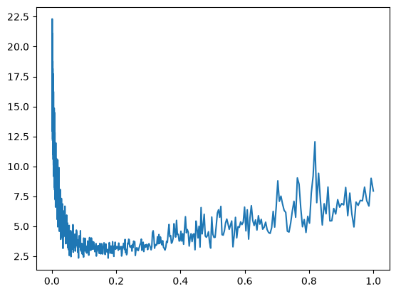
# often our plot looks like this
# initially due to low learning rate, barely anything happens
# then we get to nice spot like at that intersection between vertical and horizontal lines of L
# then as we increased the learning rate way too much, it started to become very unstable
# so according to that graph, a good learning rate is somewhere at around x = 0.1 or lets say 0.1-0.18 i guess
plt.plot(lre, lossi)[<matplotlib.lines.Line2D at 0x76afbefab620>]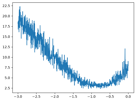
# what we want to log would be learning rate exponent instead
# x-axis: exponent of learning rate
# the exponent of the learning rate we want to use is in teh vallye at around -1.0 to -0.5
# somewhere around -1 for learning rate is a good setting, i.e. 10^(-1) = 0.1 good learning rate
# so this is roughly how we'd determine the learning rate, now we have confidence of a good learning rate
# since we're confident, we can increase our iterations by a lot
# so, we can run many examples near instantly
for i in range(10000):
# mini-batch construct
ix = torch.randint(0, X.shape[0], (32,))
# forward pass
emb = C[X[ix]] # we're only getting 32 rows of X instead of all rows of X. So embeddings will still be 32x3x2
h = torch.tanh(emb.view(-1,6) @ W1 + b1) #32 x 100
logits = h @ W2 + b2 #32 x 27
loss = F.cross_entropy(logits, Y[ix])
# print(loss.item())
# backward pass
# 1. we want to set the gradients to be 0
for p in parameters:
p.grad = None
loss.backward() #populate the gradients
# parameter update via gradients
lr = 10**(-1)#just write 0.1 lol
for p in parameters:
p.data += (-lr) * p.grad
# track stats
lri.append(lr)
lossi.append(loss.item())emb = C[X] # we're only getting 32 rows of X instead of all rows of X. So embeddings will still be 32x3x2
h = torch.tanh(emb.view(-1,6) @ W1 + b1) #32 x 100
logits = h @ W2 + b2 #32 x 27
loss = F.cross_entropy(logits, Y)
print(loss.item())2.4095613956451416
# after running it for 3 times, when we sense it is in a state of plateau, now we're going to do learning rate decay
# we're going to 10x lower our learning rate at late stages of training potentially
# note: why 10x? this is also hard to find, but eh for now just for estimated randomly
# bigram loss: 2.45, so we've already surpassed the bigram model# so, we can run many examples near instantly
for i in range(10000):
# mini-batch construct
ix = torch.randint(0, X.shape[0], (32,))
# forward pass
emb = C[X[ix]] # we're only getting 32 rows of X instead of all rows of X. So embeddings will still be 32x3x2
h = torch.tanh(emb.view(-1,6) @ W1 + b1) #32 x 100
logits = h @ W2 + b2 #32 x 27
loss = F.cross_entropy(logits, Y[ix])
# print(loss.item())
# backward pass
# 1. we want to set the gradients to be 0
for p in parameters:
p.grad = None
loss.backward() #populate the gradients
# parameter update via gradients
lr = 10**(-2)#just write 0.01 lol
for p in parameters:
p.data += (-lr) * p.grad
# track stats
lri.append(lr)
lossi.append(loss.item())emb = C[X] # we're only getting 32 rows of X instead of all rows of X. So embeddings will still be 32x3x2
h = torch.tanh(emb.view(-1,6) @ W1 + b1) #32 x 100
logits = h @ W2 + b2 #32 x 27
loss = F.cross_entropy(logits, Y)
print(loss.item())2.3289268016815186
# wow, we achieved a nice low rate
# but this is not how it is done in production
# first find decent learning rate as shown above, then train with that learning rate for a while,
# then decay the learning rate by eg. a factor of 10, and do a few more steps
# then you get a roughly trained network
# note: saying that our model is better because the loss is lower is not exactly true
# currently our neural net has 3481 parameters, but it could have 10,000 or even 100,000 parameters or more
# as the capacity of neural network grows, it becomes more and more capable of overfitting our training set
# i.e. loss on the training set's data will become as low as zero
# but our model will just be memorizing our training set verbatim (word for word)# so you may feel that the model is working really well, and when you try to sample from it
# you'll get examples exactly as they are in the training set instead of new data
# and if you try to evaluate the loss with other words not in training but correct words, the loss will be very high
# so overtraining is also not a good modelTraining, validation and test sets
# a good standard is to split our dataset into: train split, dev/validation split and test split
# roughly 80% train, 10% dev/ 10% test
# the 80% of data is used to optimize the parameters of the model using gradient descent
# 10% of dev split is used for development over all the hyperparameters of the model
# hyperparameters: we get to determine, in our eg. size of hidden layer, size of input embedding, or strength of regularization
# at the end: test split: evaluate the performance of the model
# we evaluate the loss on the test split very sparingly and very few times
# cuz every time we evaluate our test loss, and you learn something from it, you're also starting to train on the test split
# i.e. risk of overfitting as you experiment your model too
Now, lets split our dataset into train, dev and test datasets
# build the dataset

def build_dataset(words):
    block_size = 3 # context length: how many characters to take as input to predict the single next character? #taking 3 cuz it's in paper though its for words
    X, Y = [], [] #X: input to neural net, Y: labels/outputs for each example inside X
    for w in words:
        context = [0] * block_size #start with padded context of just '0' tokens
        for ch in w + '.':
            ix = stoi[ch]#get the next character in sequence
            X.append(context) #the current 3 characters
            Y.append(ix) #the next character
            # print(''.join(itos[i] for i in context), '--->', itos[ix])
            context = context[1:] + [ix] #crop and append, like a rolling window of context

    X = torch.tensor(X)
    Y = torch.tensor(Y)
    print(X.shape, Y.shape)
    return X, Y

import random
random.seed(42)
random.shuffle(words)
n1 = int(0.8 * len(words))
n2 = int(0.9 * len(words))
print(n1, n2)

Xtr, Ytr = build_dataset(words[:n1])#say len(words) = 100, 0-80
Xdev, Ydev = build_dataset(words[n1:n2])#80-90
Xte, Yte = build_dataset(words[n2:])#90-100
25626 28829
torch.Size([182580, 3]) torch.Size([182580])
torch.Size([22767, 3]) torch.Size([22767])
torch.Size([22799, 3]) torch.Size([22799])
#
print(n1) #count of training examples
print(n2-n1) #count of dev examples
print(len(words) - n2) #count of test examples
# in above mismatch cuz that's individual examples made from the words
25626
3203
3204
# first, let's reset our network parameters
# dataset
print(Xtr.shape, Ytr.shape)

g = torch.Generator().manual_seed(2147483647)
C = torch.randn((27, 2), generator=g)
W1 = torch.randn((6, 100), generator=g)
b1 = torch.randn(100, generator=g)
W2 = torch.randn((100, 27), generator=g)
b2 = torch.randn(27, generator=g)
parameters = [C, W1, b1, W2, b2]

# total number of parameters
print(sum(p.nelement() for p in parameters))

for p in parameters:
    p.requires_grad = True
torch.Size([182580, 3]) torch.Size([182580])
3481
for i in range(30000):

    # mini-batch construct
    ix = torch.randint(0, Xtr.shape[0], (32,))

    # forward pass
    emb = C[Xtr[ix]] # we're only getting 32 rows of X instead of all rows of X. So embeddings will still be 32x3x2
    h = torch.tanh(emb.view(-1,6) @ W1 + b1) #32 x 100
    logits = h @ W2 + b2 #32 x 27
    loss = F.cross_entropy(logits, Ytr[ix])
    # print(loss.item())

    # backward pass
    # 1. we want to set the gradients to be 0
    for p in parameters:
        p.grad = None
    loss.backward() #populate the gradients

    # parameter update via gradients
    lr = 10**(-1)#just write 0.1 lol
    for p in parameters:
p.data += (-lr) * p.gradprint(loss.item())2.5150628089904785
# and when we evaluate, let's use the dev instead of train
emb = C[Xdev] # we're only getting 32 rows of X instead of all rows of X. So embeddings will still be 32x3x2
h = torch.tanh(emb.view(-1,6) @ W1 + b1) #32 x 100
logits = h @ W2 + b2 #32 x 27
loss = F.cross_entropy(logits, Ydev)
loss
tensor(2.3566, grad_fn=<NllLossBackward0>)# hmm, this loss is pretty decent despite the model having not seen the examples
# lets look it for training data too# and when we evaluate, let's use the dev instead of train
emb = C[Xtr] # we're only getting 32 rows of X instead of all rows of X. So embeddings will still be 32x3x2
h = torch.tanh(emb.view(-1,6) @ W1 + b1) #32 x 100
logits = h @ W2 + b2 #32 x 27
loss = F.cross_entropy(logits, Ytr)
losstensor(2.3513, grad_fn=<NllLossBackward0>)# since the training and the dev loss are equal, we're not overfitting
# the model isn't powerful enough to purely memorize the data
# actually, we're underfitting as training loss and dev losses are roughly equal, it means our network is very small
# so, we expect to improve training performance by scaling the size of the neural netIncreasing capacity
Lets increase the size of the neural net now.
Our hidden layer has 100 neurons, lets do 300# first, let's reset our network parameters
# dataset
print(Xtr.shape, Ytr.shape)
g = torch.Generator().manual_seed(2147483647)
C = torch.randn((27, 2), generator=g)
W1 = torch.randn((6, 300), generator=g)
b1 = torch.randn(300, generator=g)
W2 = torch.randn((300, 27), generator=g)
b2 = torch.randn(27, generator=g)
parameters = [C, W1, b1, W2, b2]
# total number of parameters
print(sum(p.nelement() for p in parameters))
for p in parameters:
p.requires_grad = Truetorch.Size([182580, 3]) torch.Size([182580])
10281
# note: 10000+ parameters instead of 3000+lossi = []
stepi = []
for i in range(40000):
# mini-batch construct
ix = torch.randint(0, Xtr.shape[0], (32,))
# forward pass
emb = C[Xtr[ix]] # we're only getting 32 rows of X instead of all rows of X. So embeddings will still be 32x3x2
h = torch.tanh(emb.view(-1,6) @ W1 + b1) #32 x 100
logits = h @ W2 + b2 #32 x 27
loss = F.cross_entropy(logits, Ytr[ix])
# print(loss.item())
# backward pass
# 1. we want to set the gradients to be 0
for p in parameters:
p.grad = None
loss.backward() #populate the gradients
# parameter update via gradients
lr = 10**(-2)#just write 0.1 lol
for p in parameters:
p.data += (-lr) * p.grad
# track stats
stepi.append(i)
lossi.append(loss.item())plt.plot(stepi, lossi)[<matplotlib.lines.Line2D at 0x76afbff2d400>]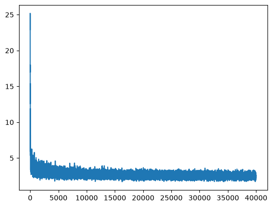
# the graph above shows how the loss function is being optimized
# btw, the graph looks like that only on first run, on later runs it will probably be more straight
# the thickness is because we're optimizing over mini-batches, and the mini-batches create a little bit of noise# one possibility: our batch size is too low: currently 32 low, so we have much noise in the training
# to prevent thrashing and gain stability, you can increase batch size# and when we evaluate, let's use the dev instead of train
emb = C[Xdev] # we're only getting 32 rows of X instead of all rows of X. So embeddings will still be 32x3x2
h = torch.tanh(emb.view(-1,6) @ W1 + b1) #32 x 100
logits = h @ W2 + b2 #32 x 27
loss = F.cross_entropy(logits, Ydev)
print(loss)tensor(2.2139, grad_fn=<NllLossBackward0>)
# and when we evaluate, let's use the dev instead of train
emb = C[Xtr] # we're only getting 32 rows of X instead of all rows of X. So embeddings will still be 32x3x2
h = torch.tanh(emb.view(-1,6) @ W1 + b1) #32 x 100
logits = h @ W2 + b2 #32 x 27
loss = F.cross_entropy(logits, Ytr)
losstensor(2.1985, grad_fn=<NllLossBackward0>)# its at 2.42, repeat the process to minimize loss
# after getting around 2.32, learning rate decay
# do it some times, then we decreased the learning rate
# wow, got a 2.20, 2.21
# our expectation is to get lower loss than before, increasing the size of neural net to prevent underfitting
# after multiple multiple iterations even after learning rate decay, got approximately around 2.2 and it didn't go lower than that# one bottleneck that might be in our network right now is that the embeddings are just 2 dimensional
# we're cramming way too many characters into just 2 dimensions# after training, we can visualize the embedding vectors for the characters, but its possible to visualize only cuz dimension size = 2
# we want to see similar characters togetherplt.figure(figsize=(8,8))
plt.scatter(C[:,0].data, C[:,1].data, s=200) #x and y-coordinates that are columns of lookup table C
for i in range(C.shape[0]):
plt.text(C[i,0].item(), C[i,1].item(), itos[i], ha="center", va="center", color='white')#also included text for each char
plt.grid('minor')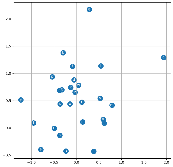
# the network has learned to cluster characters a little bit
# note that a, e, i, o, u are kind of together, y is slightly near them
# then charcters like q are very far cuz they are not so commonly used. q has special embedding c
# neural net treats a, e, i, o, u as very similar and thus interchangeable
# and other similar interchangeable letters are clustered up
# these clustering formed after training are not random and they make sense# now, we'll scale up the embedding sizeprint(Xtr.shape, Ytr.shape)
g = torch.Generator().manual_seed(2147483647)
C = torch.randn((27, 10), generator=g) #10-dimensional embeddings for each character
W1 = torch.randn((30, 250), generator=g) #this layer will receive 3(sets)x10(embeddings in each set) inputs
b1 = torch.randn(250, generator=g)
W2 = torch.randn((250, 27), generator=g)
b2 = torch.randn(27, generator=g)
parameters = [C, W1, b1, W2, b2]
# total number of parameters
print(sum(p.nelement() for p in parameters))
for p in parameters:
p.requires_grad = Truetorch.Size([182580, 3]) torch.Size([182580])
14797
lossi = []
stepi = []
for i in range(50000):
# mini-batch construct
ix = torch.randint(0, Xtr.shape[0], (32,))
# forward pass
emb = C[Xtr[ix]] # we're only getting 32 rows of X instead of all rows of X. So embeddings will still be 32x3x2
h = torch.tanh(emb.view(-1,30) @ W1 + b1) #32 x 100 #replace 3x2=6 with 3x10=30
logits = h @ W2 + b2 #32 x 27
loss = F.cross_entropy(logits, Ytr[ix])
# print(loss.item())
# backward pass
# 1. we want to set the gradients to be 0
for p in parameters:
p.grad = None
loss.backward() #populate the gradients
# parameter update via gradients
lr = 10**(-2)#just write 0.1 lol
for p in parameters:
p.data += (-lr) * p.grad
# track stats
stepi.append(i)
lossi.append(loss.log10().item())#append log of loss instead# and when we evaluate, let's use the dev instead of train
emb = C[Xdev] # we're only getting 32 rows of X instead of all rows of X. So embeddings will still be 32x3x2
h = torch.tanh(emb.view(-1,30) @ W1 + b1) #32 x 100
logits = h @ W2 + b2 #32 x 27
loss = F.cross_entropy(logits, Ydev)
print(loss)tensor(2.1580, grad_fn=<NllLossBackward0>)
# and when we evaluate, let's use the dev instead of train
emb = C[Xtr] # we're only getting 32 rows of X instead of all rows of X. So embeddings will still be 32x3x2
h = torch.tanh(emb.view(-1,30) @ W1 + b1) #32 x 100
logits = h @ W2 + b2 #32 x 27
loss = F.cross_entropy(logits, Ytr)
loss
tensor(2.0982, grad_fn=<NllLossBackward0>)# when we plot the loss, it can have the hockey stick appearance, so log squashes it inplt.plot(stepi, lossi)[<matplotlib.lines.Line2D at 0x76afaca92270>]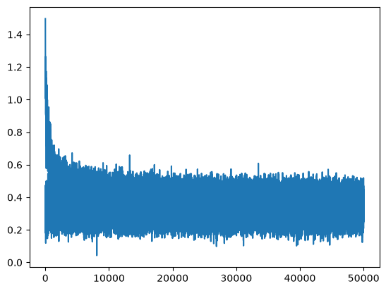
# after few steps we got 2.35(dev), 2.28(train) repeating again and again
# then we decrease the learning rate by a factor of 10 and train again
# our hope is to beat the average of 2.2 received earlier
# after decay i.e. set rate to 0.01, got 2.15 and 2.10, then 2.15 and 2.09
# but our approach is kinda haphazard, eg. learning rate decay of a factor of 10 is also random
# in production, we would create hyperparameters of all these settings, then run lots of experiments to see which ones give best dev performance
# then once you find all hyper parameters that make your dev performance good, you take that model and evaluate the test set performance a single time
# and thaaat's the number that you report in your paper or wherever else you want to brag about your model# after lots of training runs, we'll notice that the training and validation performance are starting to slowly depart
# this shows that the neural net is good enough that we are slowly starting to overfit
# since we got lower loss of 2.15 or 2.10 from 2.2, it shows that embedding size was infact holding us back# what next? we can continue to tune the optimization, play with size of neural net
# or increase the num of characters that we're taking as input, i.e. instead of 3 chars, take more which would improve the loss# andrej ran it again,
# he set learning rate like this:
# lr = 0.1 if i < 100000 else 0.01, remaining code all same
# the best validation loss he obtained was 2.17
# hmm, our validation loss was 2.15 probably cuz we used 250 neurons in hidden layer, while he used 200 neurons, cuz that's the only difference right now
# what you can change: no of neurons in hidden layer, dimensionality of embedding lookup table, no of char given as context into the model,
# you can also tune learning rate, no of iterations, decay,
# batch size(currently 32), this is probably holding things back a lot, changing this might speed up convergence speed
# read the paper, you should be able to read a good chunk of the paper
# the paper has additional ideas for improvements too# Now, lets see how we would sample from the model
# the most important part lol, seeing the actual outputInspecting and sampling the trained model
C[torch.tensor([context])].shapetorch.Size([1, 3, 10])# you might think where is the trained model being used
# look at table C whose embeddings are properly organized
# W1, b1, W2, b2, etc. we are using the latest parameters to make new predictions that give new logits, probs# sample from the model
g = torch.Generator().manual_seed(2147483647 + 10)
block_size = 3
# we'll generate 20 samples
for _ in range(20):
out = []
context = [0] * block_size #initialized with ...
while True:
emb = C[torch.tensor([context])] #embed the current context
# (1, block_size, d). 1: generating 1 eg for simplicity so 1 instead of size of training set
h = torch.tanh(emb.view(1, -1) @ W1 + b1)
logits = h @ W2 + b2
probs = F.softmax(logits, dim=1) #exponentiates the logits and makes them sum to 1, similar to cross_entropy, it is careful of no overflows
ix = torch.multinomial(probs, num_samples = 1, generator = g).item()
context = context[1:] + [ix] #shift context window to append the index
out.append(ix)
if ix == 0: #repeat until we generate the 0th character
break
print(''.join(itos[i] for i in out))carmahfamelle.
khi.
myli.
thiyah.
cassie.
mahnen.
delynn.
jareei.
nellana.
chaiir.
kaleigh.
ham.
joce.
quintis.
lilea.
jadai.
wajeangiearisi.
jace.
pirra.
med.
# the words here are much better eg. lilea, cassie, ham, jace
# so we have some progress, but we can improve on this a lot