Backpropagation by hand
Original study notes by Satish Bajagain, following Andrej Karpathy’s Zero to Hero. Comments, intermediate attempts and saved outputs are retained. Section titles are navigation additions.
Why understand the backward pass?
# we have a pretty decent understanding of the architecture of MLP
# but we are using loss.backward() directly as we should
# but what we want to do is remove loss.backward() and instead write our entire backward pass manually on the level of tensors
# but why? backprop: leaky abstraction
# its not that we can just stack up differential operations and hope our backward pass works
# sometimes, it might not work, or it might not work optimally, and you might want to know how it works under the hood if you want to debug it
# look at blog post
# flat tails of functions, you don't want to saturate them too much else the gradients will die: vanishing gradient case earlier discussed
# case of dead neurons
# and a bug that shows that the author doesn't understand backpropagation
# author tried to clip the loss at a certain max value, but they were hoping to clip the gradients at a maximum value instead
# causing outliers to be ignored cuz when you clip the loss of an outlier, you set its gradient to zero# its just that if you know stuffs, you will avoid issues in the future# we already covered autograd, and had written micrograd in lecture 1 itself
# but micrograd was an autograd engine only on the level of individual scalars
# we want to think of backprop on the level of tensors as well
# we want to better understand neural networks, what we do, and be better debuggers too
# we don't have to be nervous about what is hidden, its a good exercise too# Today, writing backward pass by hand is not recommended, and no one does it
# but it was pervasive 10 yrs ago and standard to do backward pass by hand, he showed some research papers and examples of about 10 years ago
# after doing backward pass manually, we would use a gradient checker to make sure that the numerical estimate of the gradient
# agrees with the calculated gradient during actual backprop
# but today it is standard to use autograd engine# so we're starting off where we left off last time, but instead of loss.backward(), we're going to do everything manually instead
# the only thing we're gonna use from pytorch will be torch.tensor to make everything efficientDataset and gradient checks
import torch
import torch.nn.functional as F
import matplotlib.pyplot as plt
%matplotlib inline
# read all words
words = open("names.txt", "r").read().splitlines()
print(words[:8])
print(len(words))['emma', 'olivia', 'ava', 'isabella', 'sophia', 'charlotte', 'mia', 'amelia']
32033
# Build the vocabulary of characters and mappings to/from integers
chars = sorted(list(set(''.join(words))))
stoi = {s : i+1 for i, s in enumerate(chars)}
stoi['.'] = 0
itos = {i:s for s, i in stoi.items()}
vocab_size = len(itos)
print(itos)
print(vocab_size)
{1: 'a', 2: 'b', 3: 'c', 4: 'd', 5: 'e', 6: 'f', 7: 'g', 8: 'h', 9: 'i', 10: 'j', 11: 'k', 12: 'l', 13: 'm', 14: 'n', 15: 'o', 16: 'p', 17: 'q', 18: 'r', 19: 's', 20: 't', 21: 'u', 22: 'v', 23: 'w', 24: 'x', 25: 'y', 26: 'z', 0: '.'}
27
# build the dataset
# context length: how many characters do we take to predict the next one?
block_size = 3

def build_dataset(words):
    X, Y = [], []

    for w in words:
        context = [0] * block_size
        for ch in w + '.':
            ix = stoi[ch]
            X.append(context)
            Y.append(ix)
            context = context[1:] + [ix] #crop on left and append

    X = torch.tensor(X)
    Y = torch.tensor(Y)
    print(X.shape, Y.shape)
    return X, Y

import random
random.seed(42)
random.shuffle(words)
n1 = int(0.8 * len(words))
n2 = int(0.9 * len(words))

Xtr, Ytr = build_dataset(words[:n1]) #80%
Xdev, Ydev = build_dataset(words[n1:n2]) #10%
Xte, Yte = build_dataset(words[n2:]) #10%
torch.Size([182625, 3]) torch.Size([182625])
torch.Size([22655, 3]) torch.Size([22655])
torch.Size([22866, 3]) torch.Size([22866])
# Now that boilerplate is done, we get to the action# utility function used when comparing our manual gradients to pytorch gradients
# dt: value calculated by us, t.grad: value calculated by pytorch
def cmp(s, dt, t):
ex = torch.all(dt == t.grad).item() #makes sure that every single item is equal, and converting it into a single boolean value, ex: exactly equal
app = torch.allclose(dt, t.grad) #but they might be approximately equal due to floating point issues, so are close to one another
maxdiff = (dt - t.grad).abs().max().item()
print(f'{s:15s} | exact: {str(ex):5s} | approximate: {str(app):5s} | maxdiff: {maxdiff}')Breaking the forward pass into steps
# MLP revisited
n_embd = 10 #dimensionality of the character embedding vectors
n_hidden = 64 #number of neurons in hidden layer of MLP

g = torch.Generator().manual_seed(2147483647) #use same seed for reproducibility
C = torch.randn((vocab_size, n_embd), generator = g) #embedding table for our characters

# Layer 1
W1 = torch.randn((n_embd * block_size, n_hidden), generator = g) * (5/3)/((n_embd * block_size)**0.5)
b1 = torch.randn(n_hidden, generator = g) * 0.1 #though b1 is useless because of batch norm later, using it regardless to see backprop working and gradient flow

# Layer 2
W2 = torch.randn((n_hidden, vocab_size), generator = g) * 0.1
b2 = torch.randn(vocab_size, generator = g) * 0.1

# BatchNorm parameters
bngain = torch.randn((1, n_hidden)) * 0.1 + 1.0
bnbias = torch.randn((1, n_hidden)) * 0.1

# Note: currently, we're initializing most of these parameters in non-standard ways
# normally, we'd set biases to be 0 initially, but now its small num
# cuz eg. initializing sometimes with all 0's could mask an incorrect implementation(errors) of a backward pass
# i.e. when all 0's, it simplifies, we have much simpler expression of gradient than what it would normally be

parameters = [C, W1, b1, W2, b2, bngain, bnbias]
print(sum(p.nelement() for p in parameters))
for p in parameters:
    p.requires_grad = True
4137
batch_size = 32
n = batch_size # a shorter variable for convenience

# construct a minibatch
ix = torch.randint(0, Xtr.shape[0], (batch_size, ), generator=g)
Xb, Yb = Xtr[ix], Ytr[ix] #batch X, Y
# old implementation
# # forward pass
# emb = C[Xb] #embed the characters into vectors
# embcat = emb.view(emb.shape[0], -1) #concatenate the vectors
# # Linear layer
# hpreact = embcat @ W1 # + b1 #hidden layer pre-activation #will be roughly unit Gaussian in the first iteration #removed b1 from here and above parameters list too
# # Batch normalization (batchnorm) layer
# # ----------------------------------------------------------------------------------------------------------------------------------
# bnmeani = hpreact.mean(0, keepdim=True) #batch normalization mean for the ith iteration #will be roughly 0 for the first iteration
# bnstdi = hpreact.std(0, keepdim=True) #will be roughly 1 for the first iteration
# hpreact = bngain * (hpreact - bnmeani) / bnstdi + bnbias
# # we don't want pytorch to build a graph for update of mean/sd
# # this update is separate than the gradient based optimization during backprop
# with torch.no_grad():
# # it will be mostly what it already is, but receive a small update based on the direction of what the current mean/sd is
# bnmean_running = 0.999 * bnmean_running + 0.001 * bnmeani
# bnstd_running = 0.999 * bnstd_running + 0.001 * bnstdi
# # ----------------------------------------------------------------------------------------------------------------------------------
# # non-linearity
# h = torch.tanh(hpreact) #hidden layer
# logits = h @ W2 + b2 #output layer
# loss = F.cross_entropy(logits, Yb) #loss function
# # backward pass
# for p in parameters:
# p.grad = None
# loss.backward()# forward pass but chunkated into smaller steps that are possible to backward one at a time
emb = C[Xb] #embed the characters into vectors
embcat = emb.view(emb.shape[0], -1) #concatenate the vectors
# Linear Layer 1
hprebn = embcat @ W1 + b1 #hidden layer pre-activation
# Batch normalization (batchnorm) layer
bnmeani = (1 / n) * (hprebn.sum(0, keepdim=True))
bndiff = hprebn - bnmeani
bndiff2 = bndiff**2
bnvar = (1/(n-1)) * (bndiff2).sum(0, keepdim=True) #note: Bessel's correction (dividing by n-1, not n)
bnvar_inv = (bnvar + 1e-5)**-0.5
bnraw = bndiff * bnvar_inv
hpreact = bngain * bnraw + bnbias
# Non-linearity
h = torch.tanh(hpreact) #hidden layer
# Linear Layer 2
logits = h @ W2 + b2 #output layer
# explicitly implementing loss function instead of calling cross_entropy
# cross entropy loss: same as loss = F.cross_entropy(logits, Yb)
logit_maxes = logits.max(1, keepdim=True).values
norm_logits = logits - logit_maxes #subtract max for numerical stability
counts = norm_logits.exp()
counts_sum = counts.sum(1, keepdims=True)
counts_sum_inv = counts_sum ** -1 #for some reason, doing 1/counts_sum can't get backprop to be a bit exact, problem in pytorch's backward pass implementation of division
probs = counts * counts_sum_inv
logprobs = probs.log()
loss = -logprobs[range(n), Yb].mean()#loss function
# same as loss = F.cross_entropy(logits, Yb)
# pytorch backward pass:
for p in parameters:
p.grad = None
for t in [logprobs, probs, counts, counts_sum, counts_sum_inv,
norm_logits, logit_maxes, logits, h, hpreact, bnraw,
bnvar_inv, bnvar, bndiff2, bndiff, hprebn, bnmeani,
embcat, emb]:
t.retain_grad()
loss.backward()
losstensor(3.3284, grad_fn=<NegBackward0>)from graphviz import Digraph
from IPython.display import display
dot = Digraph("Forward Pass")
dot.attr(rankdir="LR", fontsize="12")
# Inputs
dot.node("Xb", "Xb")
dot.node("C", "C")
# Embedding
dot.node("emb", "emb")
dot.node("embcat", "embcat")
dot.edge("Xb", "emb")
dot.edge("C", "emb")
dot.edge("emb", "embcat")
# Linear 1
dot.node("W1", "W1")
dot.node("b1", "b1")
dot.node("hprebn", "hprebn")
dot.edge("embcat", "hprebn", label="@")
dot.edge("W1", "hprebn")
dot.edge("b1", "hprebn")
# BatchNorm
dot.node("bnmeani", "bnmeani")
dot.node("bndiff", "bndiff")
dot.node("bndiff2", "bndiff²")
dot.node("bnvar", "bnvar")
dot.node("bnvar_inv", "bnvar_inv")
dot.node("bnraw", "bnraw")
dot.node("bngain", "bngain")
dot.node("bnbias", "bnbias")
dot.node("hpreact", "hpreact")
dot.edge("hprebn", "bnmeani", label="mean")
dot.edge("hprebn", "bndiff")
dot.edge("bnmeani", "bndiff")
dot.edge("bndiff", "bndiff2")
dot.edge("bndiff2", "bnvar")
dot.edge("bnvar", "bnvar_inv")
dot.edge("bndiff", "bnraw")
dot.edge("bnvar_inv", "bnraw")
dot.edge("bnraw", "hpreact")
dot.edge("bngain", "hpreact")
dot.edge("bnbias", "hpreact")
# Tanh
dot.node("h", "h")
dot.edge("hpreact", "h", label="tanh")
# Linear 2
dot.node("W2", "W2")
dot.node("b2", "b2")
dot.node("logits", "logits")
dot.edge("h", "logits", label="@")
dot.edge("W2", "logits")
dot.edge("b2", "logits")
# Softmax/Cross-Entropy
dot.node("logit_maxes", "logit_maxes")
dot.node("norm_logits", "norm_logits")
dot.node("counts", "counts")
dot.node("counts_sum", "counts_sum")
dot.node("counts_sum_inv", "counts_sum_inv")
dot.node("probs", "probs")
dot.node("logprobs", "logprobs")
dot.node("loss", "loss")
dot.edge("logits", "logit_maxes")
dot.edge("logits", "norm_logits")
dot.edge("logit_maxes", "norm_logits")
dot.edge("norm_logits", "counts", label="exp")
dot.edge("counts", "counts_sum")
dot.edge("counts_sum", "counts_sum_inv")
dot.edge("counts", "probs")
dot.edge("counts_sum_inv", "probs")
dot.edge("probs", "logprobs", label="log")
dot.edge("logprobs", "loss")
display(dot)Loading...
Backpropagating the loss
# Exercise 1: backprop through the whole thing manually,
# backpropagating through exactly all of the variables
# as they are defined in the forward pass above, one by one

# obv dloss/dloss = 1, no need to compute it

# loss =  -logprobs[range(n), Yb].mean()
# gradient of loss w.r.t all elements of dlogprobs, i.e. dlogprobs = ???, i.e. how does logprobs influence the loss?
# logprobs.shape: 32x27
# Yb.shape : 32
# logprobs[range(n), Yb].shape: 32

# lets understand with a simpler example, its something like this but 32 instead of 3:
# loss = -(a + b + c) / 3
# dloss/da = -1/3*da/da - 1/3*db/da - 1/3*dc/da = -1/3 - 0 - 0 = -1/3
# so, dloss/dlogprobs = -1/32, but here n = size of batch = 32, so dloss/dlogprobs = -1/n, where n = batch_size = 32
# but this holds for 32 elements plucked out from logprobs, what about the other elements? logprobs is a large array: 32x27 = 867
# the remaining elements gradient or dloss/dlogprobs is 0 cuz no matter their value / change in value, it doesn't affect final loss, only these 32 elements affect final loss
# now, we have everything

# dlogprobs = torch.zeros((32,27)), would be fine, but we want to avoid hardcoding nums like 32, 27,
dlogprobs = torch.zeros_like(logprobs) #creates an entire array of all 0s exactly in the shape of logprobs
# now set the value 1/32 exactly inside the locations [range(n), Yb]
dlogprobs[range(n), Yb] = -1.0/n #this is the final derivative for logprobs

cmp('logprobs', dlogprobs, logprobs)
logprobs | exact: True | approximate: True | maxdiff: 0.0
# btw don't be confused, during coding, variable names are dlogprobs, but while computing derivatives i do dloss/dlogprobs, so variable dlogprobs = dloss/dlogprobs# logprobs = probs.log()
# dloss/dprobs = dloss/dlogprobs * dlogprobs/dprobs (chain rule)
# dloss/dprobs = -1.0/n * d(probs.log())/dprobs [since d(log(x) / dx = 1/x)]
# dloss/dprobs = -1.0/n * 1/probs = -1/(n * probs)
# print(type(n)): int
# print(probs.shape): 32x27, so their multiplication would be multiply each element of probs by n=32
# dprobs = - 1.0 / (n * probs): probs | exact: False | approximate: False | maxdiff: 5.181398868560791
# wont work cuz in dlogprobs, almost every entry is 0 except for 1 entry in each row which is -1.0/n, its the whole array lil bro, why u trynna replace a tensor with a scalar
dprobs = dlogprobs * 1.0/(probs) #what's happening here is during backprop: take the character's whose probabilities are low, and boost their gradient(cuz divide)
cmp('probs', dprobs, probs)probs | exact: True | approximate: True | maxdiff: 0.0
# probs = counts * counts_sum_inv #implicit broadcasting done by pytorch here: 32x27 * 32x1
# trying to do probs = counts/counts.sum(1, keepdims=True), after exponentiating logits, normalize the counts to get probability distribution

# dloss/dcounts_sum_inv = dloss/dprobs * dprobs/dcounts_sum_inv
# dloss/dcounts_sum_inv = dprobs(computed above) * d(counts * counts_sum_inv)/dcounts_sum_inv
# dloss/dcounts_sum_inv = dprobs * counts * dcounts_sum_inv/dcounts_sum_inv = dprobs * counts

# print(counts.shape, counts_sum_inv.shape)
# dcounts_sum_inv = dprobs * counts

# why didn't this work? let's understand with example:
# c = a * b but with tensors:
# a[3x3] x b[3x1] = c[3x3]
# a11xb1 a12xb1 a13xb1
# a21xb2 a22xb2 a23xb2
# a31xb3 a32xb3 a33xb3
# this looks like a single operation, but it is actually 2 operations: counts * counts_sum_inv:
# 1. replicate the column tensor b across all columns of a
# 2. multiplication

# lets backpropagate through multiplication first,
# dc/db = a, dc/da = b, you understand how we got dcounts_sum_inv = dprobs * counts
# the problem with this is that, we dont have a replicated b across all dimensions, it is just a single b column
# how to backpropagate through the replication
# remember from micrograd, if a node is used multiple times, the gradients from all its uses sum during backprop
# here, column b is used multiple times above in multiplication, so we need to sum it horizontally across all rows
# sum in dim 0 sums row wise, so sum in dim 1, and we want to retain the dimension so that counts_sum_inv and dcounts_sum_inv have the same shape so keepdim=True

dcounts_sum_inv = (dprobs * counts).sum(1, keepdim=True)
cmp('counts_sum_inv', dcounts_sum_inv, counts_sum_inv)
counts_sum_inv | exact: True | approximate: True | maxdiff: 0.0
counts = norm_logits.exp()
counts_sum = counts.sum(1, keepdims=True)
counts_sum_inv = counts_sum ** -1 #for some reason, doing 1/counts_sum can't get backprop to be a bit exact, problem in pytorch's backward pass implementation of division
probs = counts * counts_sum_inv
# counts_sum_inv = counts_sum ** -1
# dloss/dcounts_sum = dloss/dcounts_sum_inv * dcounts_sum_inv/dcounts_sum
# dcounts_sum = dcounts_sum_inv * d(counts_sum ** -1 )/dcounts_sum [d(-1/x)/dx = -1/(x**2)]
# dcounts_sum = dcounts_sum_inv * -1/(counts_sum ** 2)
# dcounts_sum = dcounts_sum_inv * -1/(counts_sum ** 2)#ah ah ah, andrej did say that 1/x didn't work properly before so do x**-1, using that worked lol. nice nice
dcounts_sum = dcounts_sum_inv * -(counts_sum ** 2)**-1
cmp('counts_sum', dcounts_sum, counts_sum)
dcounts_sum = (-counts_sum**-2) * dcounts_sum_inv #bro what, the inverse's multiplication sets both true, but prev had false for exact
cmp('counts_sum', dcounts_sum, counts_sum)counts_sum | exact: True | approximate: True | maxdiff: 0.0
counts_sum | exact: True | approximate: True | maxdiff: 0.0
counts.shape, counts_sum.shape(torch.Size([32, 27]), torch.Size([32, 1]))# asdfaowiue13euwoeias
# a11 a12 a13 ---> (a11 + a12 + a13 =) b1
# a21 a22 a23 ---> (a21 + a22 + a23 =) b2
# a31 a32 a33 ---> (a31 + a32 + a33 =) b3
# Here, b1 depends on a11, a12 and a13 only. so b1's derivative w.r.t them is 1, whereas b1's derivate w.r.t a21, a22, ..., a33 is 0 as it doesn't depend on them
# understand that the gradient flows horizontally from b1 to a11, a12, a13
# this is the same concept for counts.shape and counts_sum.shape. that sum column should replicate 27 times for each column of counts
# that's why we do: dcounts = torch.ones_line(counts) * dcounts_sum# probs = counts * counts_sum_inv #implicit broadcasting done by pytorch here: 32x27 * 32x1
# dloss/dcounts = dloss/dprobs * dprobs/dcounts
# (variable based)dcounts = dprobs * d(counts * counts_sum_inv)/dcounts
# (variable based)dcounts = dprobs * counts_sum_inv
# print(dprobs.shape) #32x27
# print(counts_sum_inv.shape) #32x1
# imagine similar case, here too we replicate, so sum across dim 1 and preserve dimension
# a[3x2] x b[3x1]
# a11*b1 a12*b1
# a21*b2 a22*b2
# a31*b3 a32*b3
# dcounts = (dprobs * counts_sum_inv).sum(1, keepdim=True) #no lol, this is wrong. understand why this is wrong
# we anticipated that this wouldn't work, cuz counts is also used for count_sum, we have to add that to its gradient too ok, so wait for counts_sum to complete first
# dcounts1 = (dprobs * counts_sum_inv).sum(1, keepdim=True) #why didn't this work?????
dcounts = (dprobs * counts_sum_inv)
cmp('counts', dcounts, counts)
# second part
# dloss/dcounts = dloss/dcounts_sum * dcounts_sum/dcounts
# dcounts = dcounts_sum * d(counts.sum(1, keepdims=True))/dcounts
# counts.shape #32x27
# len(counts.sum(1, keepdims=True)) #32
# d(counts.sum(1, keepdims=True))/dcounts: explanation to this is in above cell starting with asdfaowiue13euwoeias
# is it like d(a+b+c)/da = 1, then for all elements too its 1
# dcounts = dcounts_sum * d(counts.sum(1, keepdims=True))/dcounts
# dcounts = dcounts_sum * 1(yes but in the shape of counts) = dcounts_sum * torch.ones_like(counts)
dcounts += dcounts_sum * torch.ones_like(counts)
cmp('counts', dcounts, counts)counts | exact: False | approximate: False | maxdiff: 0.005950985476374626
counts | exact: True | approximate: True | maxdiff: 0.0
# counts = norm_logits.exp()
# dloss/dnorm_logits = dloss/dcounts * dcounts/dnorm_logits
# dnorm_logits = dcounts * d(norm_logits.exp())/dnorm_logits [de^x/dx = e^x]
# dnorm_logits = dcounts * norm_logits.exp()

# NICE: BTW, we are referencing above graph to determine what's derivative to find next, then after that the equation comes to be relevant
dnorm_logits = dcounts * norm_logits.exp() #since counts = norm_logits.exp(), you can replace this expression by counts * dcounts as well
cmp('norm_logits', dnorm_logits, norm_logits)
norm_logits | exact: True | approximate: True | maxdiff: 0.0
# norm_logits = logits - logit_maxes #subtract max for numerical stability
# dloss/dlogit_maxes = dloss/dnorm_logits * dnorm_logits/dlogit_maxes
# dlogit_maxes = dnorm_logits * d(logits - logit_maxes)/dlogit_maxes
# dlogit_maxes = dnorm_logits * d(logits)/dlogit_maxes - dlogit_maxes/dlogit_maxes
# dlogit_maxes = dnorm_logits * (d(logits)/dlogit_maxes - dlogit_maxes/dlogit_maxes)
# dlogit_maxes = dnorm_logits * (0 - 1)#changing logit_maxes has 0 effect on logits cuz logits is itself used to calculate logit_maxes indirectly
# dlogit_maxes = -dnorm_logits

dlogit_maxes = -dnorm_logits
cmp('logit_maxes', dlogit_maxes, logit_maxes)

# ok that didn't work, maybe something is wrong in the shape
# look at main exp: norm_logits = logits - logit_maxes
print(norm_logits.shape, logits.shape, logit_maxes.shape)

# aha, there's implicit broadcasting going on then, each of the logit_maxes is being replicated 27 times

# c11 c12 c13 = a11 a12 a13 - b1
# c21 c22 c23 = a21 a22 a23 - b2
# c31 c32 c33 = a31 a32 a33 - b3
# c11 = a11 - b1
# so, derivatives on c will flow to corresponding a's and b's
# additionally, bs are broadcast, so we have to do the sum

dlogit_maxes = (-dnorm_logits * torch.ones_like(logit_maxes)).sum(1, keepdims=True)
cmp('logit_maxes', dlogit_maxes, logit_maxes)
logit_maxes | exact: False | approximate: False | maxdiff: 0.03082321211695671
torch.Size([32, 27]) torch.Size([32, 27]) torch.Size([32, 1])
logit_maxes | exact: True | approximate: True | maxdiff: 0.0
# logit_maxes = logits.max(1, keepdim=True).values
# norm_logits = logits - logit_maxes

# dloss/dlogits = dloss/dlogit_maxes * dlogit_maxes/dlogits + dloss/dnorm_logits * dnorm_logits/dlogits

# lets do it one at a time instead, we start by checking the shape from now on

# suppose, logits = [2.0, 5.0, 3.0], then logit_maxes = [5.0], then norm_logits = [-3, 0, -2]
# if logits.shape [n, 27], logit_maxes.shape = [n, 1]
print(logit_maxes.shape, logits.shape) #ok, so we are NOT NOT NOT NOT NOT summing values in rows across all columns
# across each row, we are just plucking the maximum value in a row and assigning it.
# [a11 a12 a13] ──max──> [c11]
# [b11 b12 b13] ──max──> [c21]
# so we need to take the dlogit maxes and scatter to correct position in the logits from where the max value came: backward pass
# very similar to first example, fill with zeros and populate the elements

# for: logit_maxes = logits.max(1, keepdim=True).values
# logits = [2, 5, 3], max=5. During backward pass, if the loss changes logit_maxes by dlogit_maxes = 7, only the value that produced the maximum(here 5) should receive that gradient.
# and we set others to 0
# logits = [0, 7, 0]
# this is implemented by this code: F.one_hot(logits.max(1).indices, num_classes=logits.shape[1])
# in above case, one_hot = [0, 1, 0], then dlogit_maxes * one_hot

dlogits = dlogit_maxes * F.one_hot(logits.max(1).indices, num_classes=logits.shape[1])
cmp('logits', dlogits, logits)

# next:
# norm_logits = logits - logit_maxes #this is being done only for the stability of softmax
# remember that, when we add/subtract any num to a row in logits, the value of probs will be unchanged. its just to make sure x doesnt overflow
# that was done to ensure that the highest number would be 0, and prevent infinity from popping up
# this is why, changing logit_maxes doesn't change loss, and its gradient is 0, print (logit_maxes) to see that it is very very close to 0 as well
# lets see mathematically too
# dlogits = dnorm_logits * dnorm_logits/dlogits
# dlogits = dnorm_logits * d(logits - logit_maxes)/dlogits
# dlogits = dnorm_logits * (d(logits)/dlogits - dlogit_maxes/dlogits) #change in logits affects logit_maxes so find it
# dlogits = dnorm_logits * (1 - d(logits.max(1, keepdim=True).values)/dlogits) #we computed this recently above and did sum, so copy that mechanism here again
# focusing specially on the later part, in this case, we kinda ensure that except the max value, others get the gradients, so its mostly the same
# d(logit_maxes)/dlogits is NOT simply 0:
# only the logit that was the maximum affects logit_maxes.
#
# Example:
#     logits = [2, 5, 3]
#                  ↑ max
#
#     d(logit_max)/dlogits = [0, 1, 0]
#
# Therefore:
#
#     dnorm_logits/dlogits
#     = 1 - [0, 1, 0]
#     = [1, 0, 1]
#
# So the non-max logits get their gradient normally,
# while the max logit gets 0 from this path because:
#
#     1 - 1 = 0
#
# The gradient coming through norm_logits is therefore
# added to dlogits. The max-position adjustment is handled
# through the gradient flowing through logit_maxes.

dlogits += (dnorm_logits)

cmp('logits', dlogits, logits)
torch.Size([32, 1]) torch.Size([32, 27])
logits | exact: False | approximate: False | maxdiff: 0.03082321025431156
logits | exact: True | approximate: True | maxdiff: 0.0
# an array of where the maxes came from in each row, set that element to 1, and others to zero
plt.imshow(F.one_hot(logits.max(1).indices, num_classes=logits.shape[1]))
<matplotlib.image.AxesImage at 0x7065d2ce4440>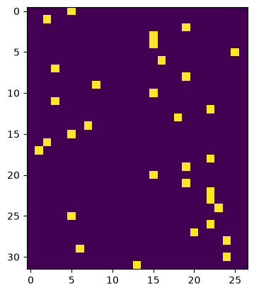
Matrix multiplication and bias
# now,
# Linear Layer 2: matrix mul + bias offset
# logits = h @ W2 + b2 #output layer: so this + is a broadcast, from the broadcast rules 27 => 1 x 27, so bias will become a row vector replicated 32 times to be 32x27
print(dlogits.shape, h.shape, W2.shape, b2.shape)

# dloss/dh = dloss/dlogits * dlogits/dh
# dh = dlogits * d(h@W2 + b2)/dh
# dh = dlogits * d(h@W2)/dh + d(b2)/dh
# dh = dlogits * W2 + 0

# dh = dlogits * W2 + 0
# cmp('h', dh, h)

# obviously this doesn't work. so you can write out a small example, and you can understand the broader pattern and write the general formula for how these derivatives flow
# LOOK AT HOW WE DERIVED THE FORMULAS TOO
# the backward pass of matrix multiplication is a matrix multiplication too
torch.Size([32, 27]) torch.Size([32, 64]) torch.Size([64, 27]) torch.Size([27])
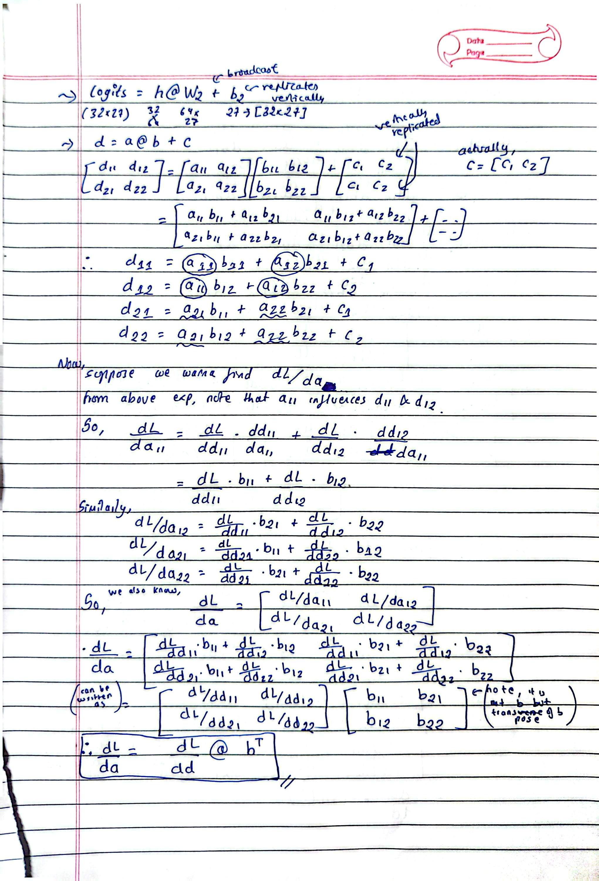
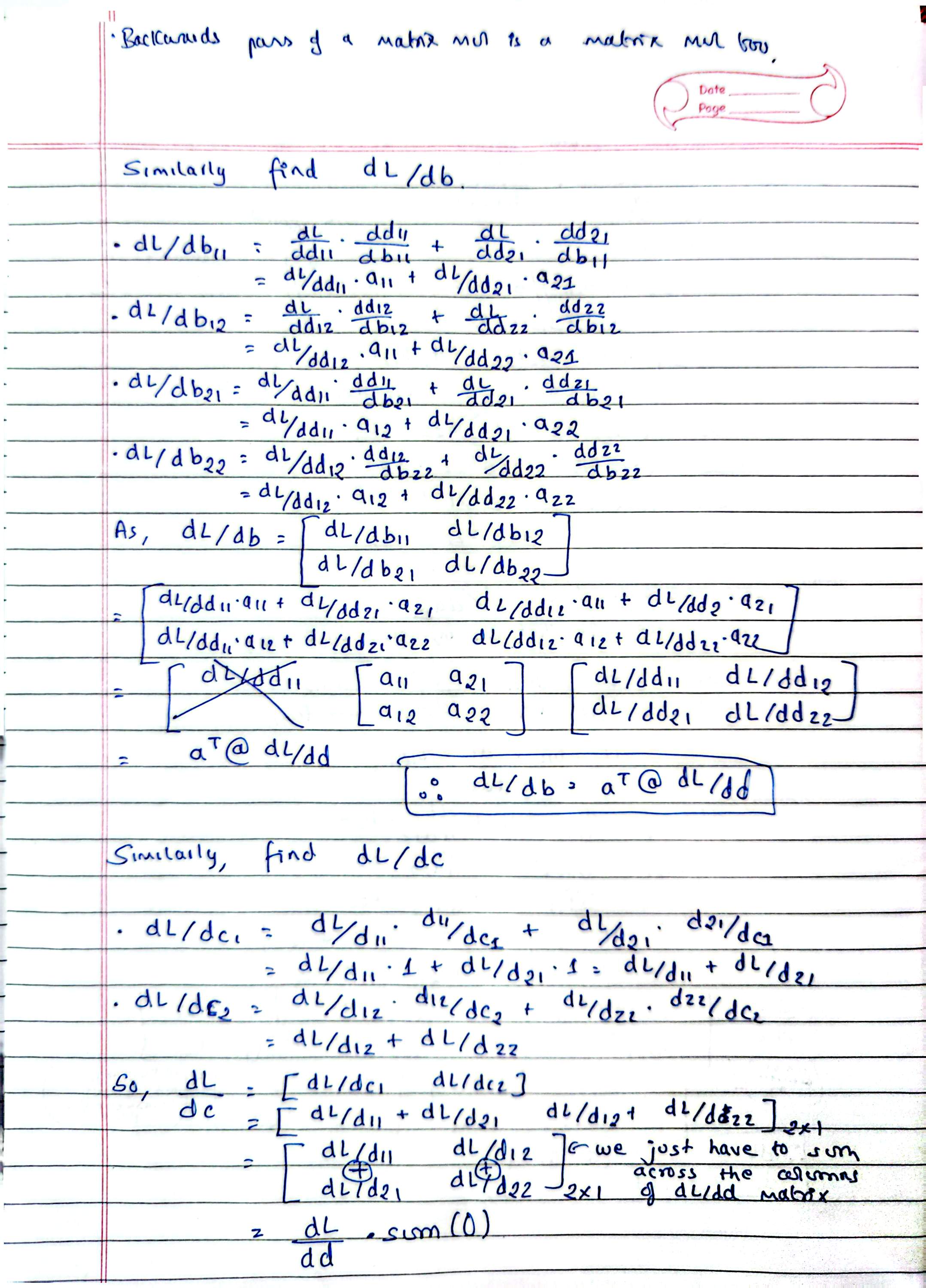
# though we worked so hard to derive these formulas, we can kinda find out the ans without them, just the dimensions have to work out
# suppose, i want to find dh. know that dh.shape must equal h.shape = 32x64
# and, h is some kind of matrix mul between dlogits and W2 (look at prev example, you'll see that finding dL/da required use of dL/dd and transpose of b)
# we have shape of dlogits: 32x27, W2: 64x27. we know that one of them must be transpose
# but since we already know the final shape of dh from h.shape, we now know exactly what the expression must be
dh = dlogits @ W2.T
# W2.T: transpose of W2 matrix
cmp('h', dh, h)
h | exact: True | approximate: True | maxdiff: 0.0
print(dlogits.shape, h.shape, W2.shape, b2.shape)
# W2.shape is 64x27, so dW2 must have the same shape as well
dW2 = h.T @ dlogits
cmp('W2', dW2, W2)
torch.Size([32, 27]) torch.Size([32, 64]) torch.Size([64, 27]) torch.Size([27])
W2 | exact: True | approximate: True | maxdiff: 0.0
print(dlogits.shape, h.shape, W2.shape, b2.shape)
# from above formula, db2 it is just sum of dlogits along the 0th dimension
# we want db2's shape to be same as b2, so its okay to collapse the dimension from 1x27 to just 27
db2 = dlogits.sum(0, keepdim=False)
cmp('b2', db2, b2)
torch.Size([32, 27]) torch.Size([32, 64]) torch.Size([64, 27]) torch.Size([27])
b2 | exact: True | approximate: True | maxdiff: 0.0
Through the nonlinearity
# that's how you backpropagate through a linear layer# h = torch.tanh(hpreact) #hidden layer
# dloss/dhpreact = dloss/dh * dh/dhpreact
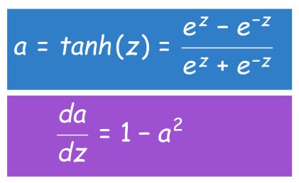
# dhpreact = dh * d(tanh(hpreact))/dhpreact (dtanx/dx = sec^2x = (cos^2x)**-1)
# dhpreact = dh * (torch.cos(hpreact)**2)**-1
# cmp('hpreact', dhpreact, hpreact)
# instead of using sec^2x, use 1 - tan^2x
# dhpreact = dh * (1.0 -(torch.tanh(hpreact)**2))
dhpreact = dh * (1.0 -(h**2))
dhpreact = (1.0 -(h**2)) * dh
cmp('hpreact', dhpreact, hpreact)#andrej got exact True too, but it doesn't matter i guesshpreact | exact: False | approximate: True | maxdiff: 4.656612873077393e-10
Through batch normalization
# this is not matrix mul, it is element-wise multiplication, need to be careful with broadcasting
print(hpreact.shape, bnraw.shape, bngain.shape, bnbias.shape)
# hpreact = bngain * bnraw + bnbias
# dloss/dbngain = dloss/dhpreact * dhpreact/dbngain
# dbngain = dhpreact * bnraw (ez to do directly), lol didn't work
# i want the output dbngain to be 1x64 since bngain is 1x64, so multiply and sum accordingly, so we set dim along 0 to sum

dbngain = (dhpreact * bnraw).sum(0, keepdim=True)
cmp('bngain', dbngain, bngain)
torch.Size([32, 64]) torch.Size([32, 64]) torch.Size([1, 64]) torch.Size([1, 64])
bngain | exact: False | approximate: True | maxdiff: 1.862645149230957e-09
# hpreact = bngain * bnraw + bnbias
# dloss/bnbias = dloss/dhpreact * dhpreact/bnbias
dbnbias = dhpreact * 1
print(hpreact.shape, bnraw.shape, bngain.shape, bnbias.shape)
dbnbias = (dhpreact).sum(0, keepdim=True) #* torch.ones_like(bnbias) inside too, same result

cmp('bnbias', dbnbias, bnbias)
torch.Size([32, 64]) torch.Size([32, 64]) torch.Size([1, 64]) torch.Size([1, 64])
bnbias | exact: False | approximate: True | maxdiff: 3.725290298461914e-09
# hpreact = bngain * bnraw + bnbias
# dbnraw = dhpreact * dhpreact/dbnraw
# dbnraw = dhpreact * bngain
print(hpreact.shape, bnraw.shape, bngain.shape, bnbias.shape)
dbnraw = dhpreact * bngain
cmp('bnraw', dbnraw, bnraw)

# really nice: you realized that this is not matrix mul, this is element wise mul
# so multiplying 32x64 with 1x64 would give 32x64 which is bnraws shape, so no need to sum, gud job
torch.Size([32, 64]) torch.Size([32, 64]) torch.Size([1, 64]) torch.Size([1, 64])
bnraw | exact: False | approximate: True | maxdiff: 9.313225746154785e-10
# Batch normalization (batchnorm) layer
bnmeani = (1 / n) * (hprebn.sum(0, keepdim=True))
bndiff = hprebn - bnmeani
bndiff2 = bndiff**2

bnvar = (1/(n-1)) * (bndiff2).sum(0, keepdim=True) #note: Bessel's correction (dividing by n-1, not n)
bnvar_inv = (bnvar + 1e-5)**-0.5 #that small value is epsilon, as you see in the formulas
bnraw = bndiff * bnvar_inv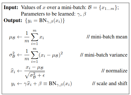
# dbnvar_inv = dbnraw * dbnraw/dbnvar_inv
# dbnvar_inv = dbnraw * d(bndiff * bnvar_inv)/dbnvar_inv
# dbnvar_inv = dbnraw * bndiff
print(bnraw.shape, bndiff.shape, bnvar_inv.shape) #desired shape is 1x64 but i think we'll get 32x64 so need to sum
# and since final has 1 row, we sum along dimension 0: i.e. along the columns
dbnvar_inv = (dbnraw * bndiff).sum(0, keepdim=True)
cmp('bnvar_inv', dbnvar_inv, bnvar_inv)
torch.Size([32, 64]) torch.Size([32, 64]) torch.Size([1, 64])
bnvar_inv | exact: False | approximate: True | maxdiff: 3.725290298461914e-09
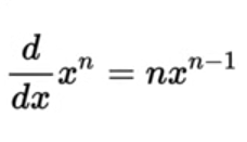
# bnvar_inv = (bnvar + 1e-5)**-0.5
# dbnvar = dbnvar_inv * dbnvar_inv/dbnvar
# dbnvar = dbnvar_inv * d((bnvar + 1e-5)**-0.5)/dbnvar
# dbnvar = dbnvar_inv * -0.5 * (bnvar + 1e-5)**(-0.5-1)

dbnvar = dbnvar_inv * -0.5 * (bnvar + 1e-5)**(-0.5-1)
cmp('bnvar', dbnvar, bnvar)
bnvar | exact: False | approximate: True | maxdiff: 4.656612873077393e-10
# bnvar = (1/(n-1)) * (bndiff2).sum(0, keepdim=True)
# lets first talk about bessel's correction, we divide by n-1 instead of n, why?
# there are two ways of estimating variance of an array,
# one is the biased estimate which is 1/n and
# the unbiased estimate which is 1/(n-1)
# its confusing in paper, train,test mismatch, they're using biased one in training, but unbiased one in inference/testing
# you can read why 1/n-1 gives a better estimate of variance, google besel's correction
# https://math.oxford.emory.edu/site/math117/besselCorrection/
# in torch.batchnorm1d also there is some bug/inconsistency about use of unbiased estimate
# this is a small problem if your mini-batch size is larger

# a11 a12 -->
# a21 a22 --> #squash the rows into a single row
# b1 b2
# b1 = (1/(n-1)) * (a11 + a21)
# b2 = (1/(n-1)) * (a12 + a22)
# we have derivatives of b1's and b2's, and we want to backpropagate them over to the a's
# so the derivative would be something like 1/(n-1) * 1 cuz b1 relies completely on a11 and a21

# dbndiff2 = dbnvar * dbnvar/dbndiff2
print(bnvar.shape, bndiff2.shape)
# dbndiff2 = dbnvar * d((1/(n-1)) * (bndiff2).sum(0, keepdim=True))/dbndiff2 #that front part is just constant, second part we have encountered so many times before
# dbndiff2 = dbnvar * (1/(n-1)) * d(bndiff2).sum(0, keepdim=True)/dbndiff2
dbndiff2 = dbnvar * (1/(n-1)) #the derivative of last part is 1 from our logic above, i finally understand it now bro
print(dbndiff2.shape, bndiff2.shape)
# but andrej did something like this which gives the same result but :
dbndiff2 = dbnvar * (1/(n-1)) * torch.ones_like(bndiff2)
print(dbndiff2.shape, bndiff2.shape)

# ah now that i think of it, i guess i have to crosscheck shapes for all prev operations too cuz i omitted x by 1 too many times
cmp('bndiff2', dbndiff2, bndiff2)
torch.Size([1, 64]) torch.Size([32, 64])
torch.Size([1, 64]) torch.Size([32, 64])
torch.Size([32, 64]) torch.Size([32, 64])
bndiff2 | exact: False | approximate: True | maxdiff: 2.9103830456733704e-11
# bnraw = bndiff * bnvar_inv
# bndiff2 = bndiff**2

# dloss/dbndiff = dloss/dbnraw * dbnraw/dbndiff
# dbndiff = dbnraw * bnvar_inv
print(bnraw.shape, bndiff.shape, bnvar_inv.shape)

dbndiff = dbnraw * bnvar_inv
cmp('bndiff', dbndiff, bndiff) #note that the diff is usually very small

# dloss/dbndiff = dloss/bndiff2 * bndiff2/dbndiff
# dbndiff += dbndiff2 * d(bndiff**2)/dbndiff [dx^2/dx = 2x]
dbndiff += dbndiff2 * 2 * bndiff
cmp('bndiff', dbndiff, bndiff)
torch.Size([32, 64]) torch.Size([32, 64]) torch.Size([1, 64])
bndiff | exact: False | approximate: False | maxdiff: 0.001129076350480318
bndiff | exact: False | approximate: True | maxdiff: 4.656612873077393e-10
# bndiff = hprebn - bnmeani
# as a hint to us because of the duality, broadcasting in forward pass means variable reuse cuz of replication, so there'll be a sum in backward pass
print(bndiff.shape, hprebn.shape, bnmeani.shape)
# dloss/dbnmeani = dloss/dbndiff * dbndiff/dbnmeani
# dbnmeani = dbndiff * d(hprebn-bnmeani)/dbnmeani
# dbnmeani = dbndiff * (0-1)
# shape of dbnmeani should be same as bnmeani, which is 1x64, so sum along dimension 0

dbnmeani = (-dbndiff * torch.ones_like(bnmeani)).sum(0, keepdim=True)
print(bnmeani.shape, dbnmeani.shape)
cmp('bnmeani', dbnmeani, bnmeani)
torch.Size([32, 64]) torch.Size([32, 64]) torch.Size([1, 64])
torch.Size([1, 64]) torch.Size([1, 64])
bnmeani | exact: False | approximate: True | maxdiff: 2.7939677238464355e-09
# bnmeani = (1 / n) * (hprebn.sum(0, keepdim=True))
# dhprebn = dbnmeani * dbnmeani/dhprebn
# dhprebn = dbnmeani * d((1 / n) * (hprebn.sum(0, keepdim=True)))/dhprebn
# dhprebn = dbnmeani * (1 / n) * d(hprebn.sum(0, keepdim=True))/dhprebn
# dhprebn = dbnmeani * (1 / n) * d(hprebn.sum(0, keepdim=True))/dhprebn
print(hprebn.shape, dbnmeani.shape)
# that sum along dimension 0 squashes all rows to 1, each value of hprebn plays a role in addition and computing of final value, so resulting derivative is 1
# but don't forget to ensure final shape is correct

dhprebn = dbnmeani * (1.0 / n) * torch.ones_like(hprebn)
print(hprebn.shape, dhprebn.shape)
cmp('hprebn', dhprebn, hprebn)

# i forgot that dhprebn was being used in 2 places, so our answer was not matching
# lol, turns out so andrej also forgot
# bndiff = hprebn - bnmeani
print(bndiff.shape, hprebn.shape, bnmeani.shape)
# dhprebn = dbndiff * dbndiff/dhprebn
# dhprebn = dbndiff * d(hprebn - bnmeani)/dhprebn
# dhprebn = dbndiff * (1-0)
dhprebn += dbndiff
cmp('hprebn', dhprebn, hprebn)
torch.Size([32, 64]) torch.Size([1, 64])
torch.Size([32, 64]) torch.Size([32, 64])
hprebn | exact: False | approximate: False | maxdiff: 0.007641538046300411
torch.Size([32, 64]) torch.Size([32, 64]) torch.Size([1, 64])
hprebn | exact: False | approximate: True | maxdiff: 4.656612873077393e-10
The first layer and embeddings
emb = C[Xb] #embed the characters into vectors
embcat = emb.view(emb.shape[0], -1) #concatenate the vectors

# Linear Layer 1
hprebn = embcat @ W1 + b1 #hidden layer pre-activation
# dloss/dembcat = dloss/dhprebn * dhprebn/dembcat
# dembcat = dhprebn * d(embcat @ W1 + b1)/dembcat
print(hprebn.shape, embcat.shape, W1.shape, b1.shape)
# dembcat.shape should equal embcat.shape, matrix multiply 2 terms (one transpose and other non-transpose to get dembcat)
dembcat = (dhprebn @ W1.T)
cmp('embcat', dembcat, embcat)torch.Size([32, 64]) torch.Size([32, 30]) torch.Size([30, 64]) torch.Size([64])
embcat | exact: False | approximate: True | maxdiff: 1.862645149230957e-09
print(hprebn.shape, embcat.shape, W1.shape, b1.shape)
dW1 = (embcat.T @ dhprebn)
cmp('W1', dW1, W1)
torch.Size([32, 64]) torch.Size([32, 30]) torch.Size([30, 64]) torch.Size([64])
W1 | exact: False | approximate: True | maxdiff: 7.450580596923828e-09
# following same pattern as previous
db1 = dhprebn.sum(0, keepdim=False)
print(b1.shape, db1.shape)
cmp('b1', db1, b1)
torch.Size([64]) torch.Size([64])
b1 | exact: False | approximate: True | maxdiff: 3.725290298461914e-09
# embcat = emb.view(emb.shape[0], -1) #concatenate the vectors from 3x10 to 30. but now we want to undo that
print(embcat.shape, emb.shape)
# view is just a logical representation of an array, just view dembcat(32x30) on basis of shape of emb (32x3x10)
demb = dembcat.view(emb.shape)
cmp('emb', demb, emb)
torch.Size([32, 30]) torch.Size([32, 3, 10])
emb | exact: False | approximate: True | maxdiff: 1.862645149230957e-09
# emb = C[Xb]
print(emb.shape, C.shape, Xb.shape)
# each one of the integers inside Xb represent which row of C we want to pluck out
# then we arrange the rows that we want to pluck out into emb: 32x3x10

dC = torch.zeros_like(C)
for k in range(Xb.shape[0]):
    for j in range(Xb.shape[1]):
        ix = Xb[k, j]
        dC[ix] += demb[k, j]
cmp('C', dC, C)
torch.Size([32, 3, 10]) torch.Size([27, 10]) torch.Size([32, 3])
C | exact: False | approximate: True | maxdiff: 5.587935447692871e-09
# Forward:
# emb = C[Xb]
#
# C is the embedding lookup table:
#     C.shape = 27 x 10
#     27 possible characters, each represented by a 10-dimensional vector.
#
# Xb contains integer indices telling us which rows of C to pick:
#     Xb.shape = 32 x 3
#     32 examples, each containing 3 character indices.
#
# Therefore:
#     emb.shape = 32 x 3 x 10
#
# Each integer Xb[k, j] tells us:
#     "take row Xb[k, j] from C and put it at emb[k, j]"
#
# Example:
#     Xb[k,j] = 11
#     => emb[k,j] = C[11]
#
# During backprop, demb contains the gradient of the loss
# with respect to every embedding that was looked up.
#
# We now need to send those gradients back to the correct rows of C.

# dC = torch.zeros_like(C)   # start with zero gradient for every row of C

# for k in range(Xb.shape[0]):       # loop through the 32 examples
#     for j in range(Xb.shape[1]):   # loop through the 3 characters
#         ix = Xb[k, j]              # which row of C was used here?

#         # Forward did:
#         #     emb[k, j] = C[ix]
#         #
#         # So backward does the reverse:
#         #     dC[ix] += demb[k, j]
#         #
#         # We ADD because the same row of C can be looked up
#         # multiple times, and all those gradients must accumulate.
#         dC[ix] += demb[k, j]

# cmp('C', dC, C)

# think of forward pass as:
# C[11] ──────→ emb[0,0]
# C[14] ──────→ emb[0,1]
# C[11] ──────→ emb[1,0]

# suppose backward pass gives:
# demb[0,0] = [a,b,c,...]
# demb[0,1] = [d,e,f,...]
# demb[1,0] = [g,h,i,...]

# then:
# dC[11] += [a,b,c,...]
# dC[14] += [d,e,f,...]
# dC[11] += [g,h,i,...]

# ultimately:
# dC[11] = [a,b,c,...] + [g,h,i,...]
# This accumulation is crucial.
# Why? Because C[11] was used twice. Both uses contributed to the final loss, so both gradient contributions must flow back into the same parameter C[11].

# Forward: C → pick rows → emb
# Backward: demb → put gradients back into those rows → dC, adding gradients when a row was used multiple times.
Cross-entropy in one step
# Exercise 2: backprop through cross_entropy but all in one go
# to complete this challenge look at the mathematical expression of the loss,
# take the derivative, simplify the expression, and just write it out

# we were doing way too much work in exercise 1, eg. F.cross_entropy was broken into so many lines but it could have been simplified

# forward pass

# before:
# logit_maxes = logits.max(1, keepdim=True).values
# norm_logits = logits - logit_maxes # subtract max for numerical stability
# counts = norm_logits.exp()
# counts_sum = counts.sum(1, keepdims=True)
# counts_sum_inv = counts_sum**-1 # if I use (1.0 / counts_sum) instead then I can't get backprop to be bit exact...
# probs = counts * counts_sum_inv
# logprobs = probs.log()
# loss = -logprobs[range(n), Yb].mean()

# now:
# h = torch.tanh(hpreact) #hidden layer
#     logits = h @ W2 + b2 #output layer
#     loss = F.cross_entropy(logits, Yb) #loss function

loss_fast = F.cross_entropy(logits, Yb)
print(loss_fast.item(), 'diff:', (loss_fast - loss).item())
3.328404188156128 diff: -2.384185791015625e-07
# # backward pass
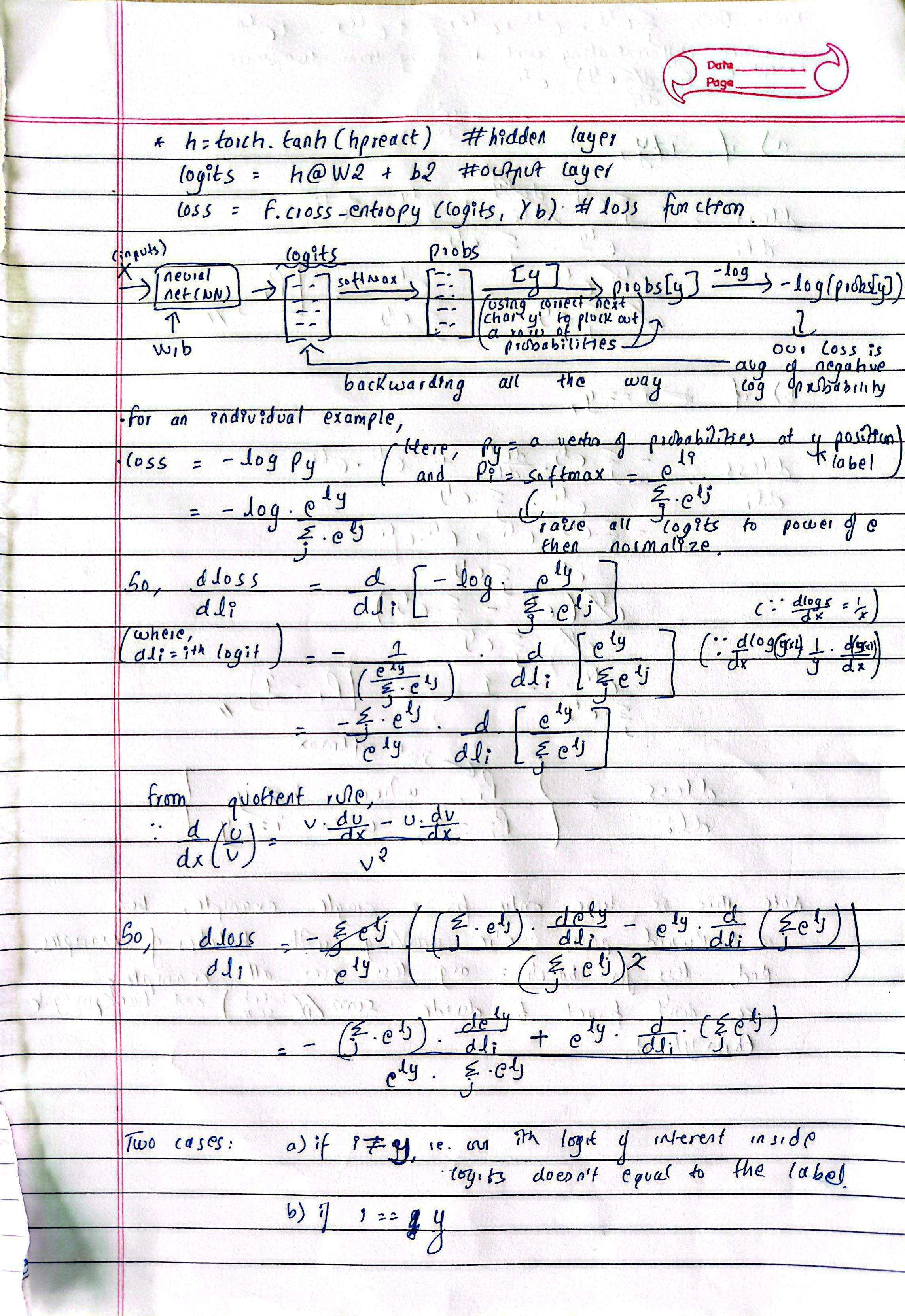
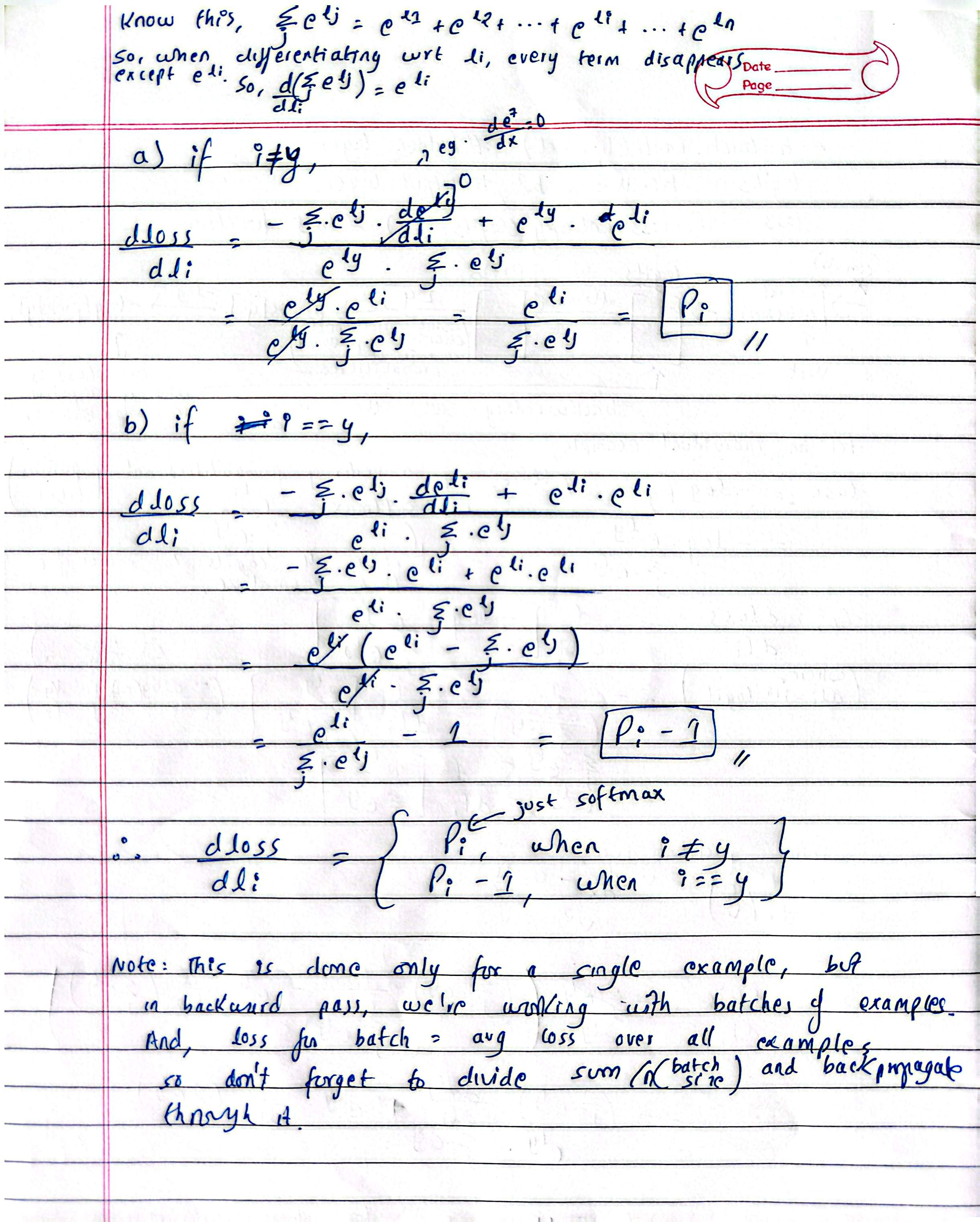
# dlogits = ???

#do the softmax across the rows of the logits
# at correct positions, subtract 1, at dlogits, iterate over all the rows, and index into columns of correct labels Yb subtract 1
# finally avg loss, 1/n
dlogits = F.softmax(logits, 1)
dlogits[range(n), Yb] -= 1
dlogits /= n

cmp('logits', dlogits, logits) # I can only get approximate to be true
logits | exact: False | approximate: True | maxdiff: 5.3551048040390015e-09
# dlogits: probabiltiies matrix in forward pass
# black square: positions of correct indices where we subtracted 1
# lets look at first row
print(F.softmax(logits,1)[0])
print(dlogits[0] * n) #the position of correct index has approximately -1
print(dlogits[0].sum()) #almost 0
tensor([0.0716, 0.0875, 0.0189, 0.0464, 0.0208, 0.0935, 0.0253, 0.0346, 0.0173,
0.0343, 0.0340, 0.0371, 0.0344, 0.0270, 0.0361, 0.0136, 0.0092, 0.0189,
0.0152, 0.0553, 0.0452, 0.0225, 0.0250, 0.0660, 0.0633, 0.0265, 0.0207],
grad_fn=<SelectBackward0>)
tensor([ 0.0716, 0.0875, 0.0189, 0.0464, 0.0208, 0.0935, 0.0253, 0.0346,
-0.9827, 0.0343, 0.0340, 0.0371, 0.0344, 0.0270, 0.0361, 0.0136,
0.0092, 0.0189, 0.0152, 0.0553, 0.0452, 0.0225, 0.0250, 0.0660,
0.0633, 0.0265, 0.0207], grad_fn=<MulBackward0>)
tensor(2.7940e-09, grad_fn=<SumBackward0>)
# The gradients act like a push-pull system on the logits:
# - the correct character is pushed UP
# - incorrect characters are pushed DOWN
#
# The total gradient sums to 0, so the amount pushed up equals
# the total amount pushed down.
#
# The strength of each push/pull is proportional to the predicted probability:
# - confidently wrong prediction -> strong push/pull
# - nearly correct prediction -> weak push/pull
# - perfectly correct prediction -> essentially no push/pull
#
# These gradients then propagate backward to the weights and biases,
# gradually "tugging" the parameters toward better predictions.
#
# This is the intuitive picture of what cross-entropy loss does
# during the backward pass.
# we want to get an intuitive sense of dlogits
plt.figure(figsize=(8,8))
print(dlogits.shape) #32 examples each having 27 chars
plt.imshow(dlogits.detach(), cmap='gray')torch.Size([32, 27])
<matplotlib.image.AxesImage at 0x7065d132f750>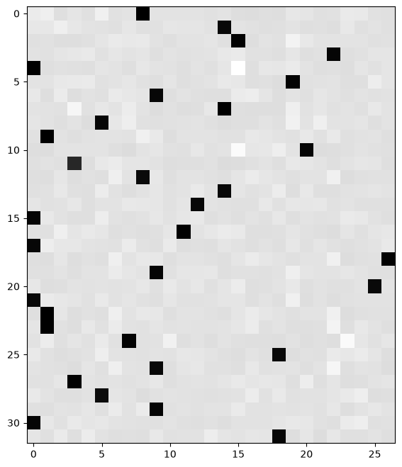
BatchNorm in one step
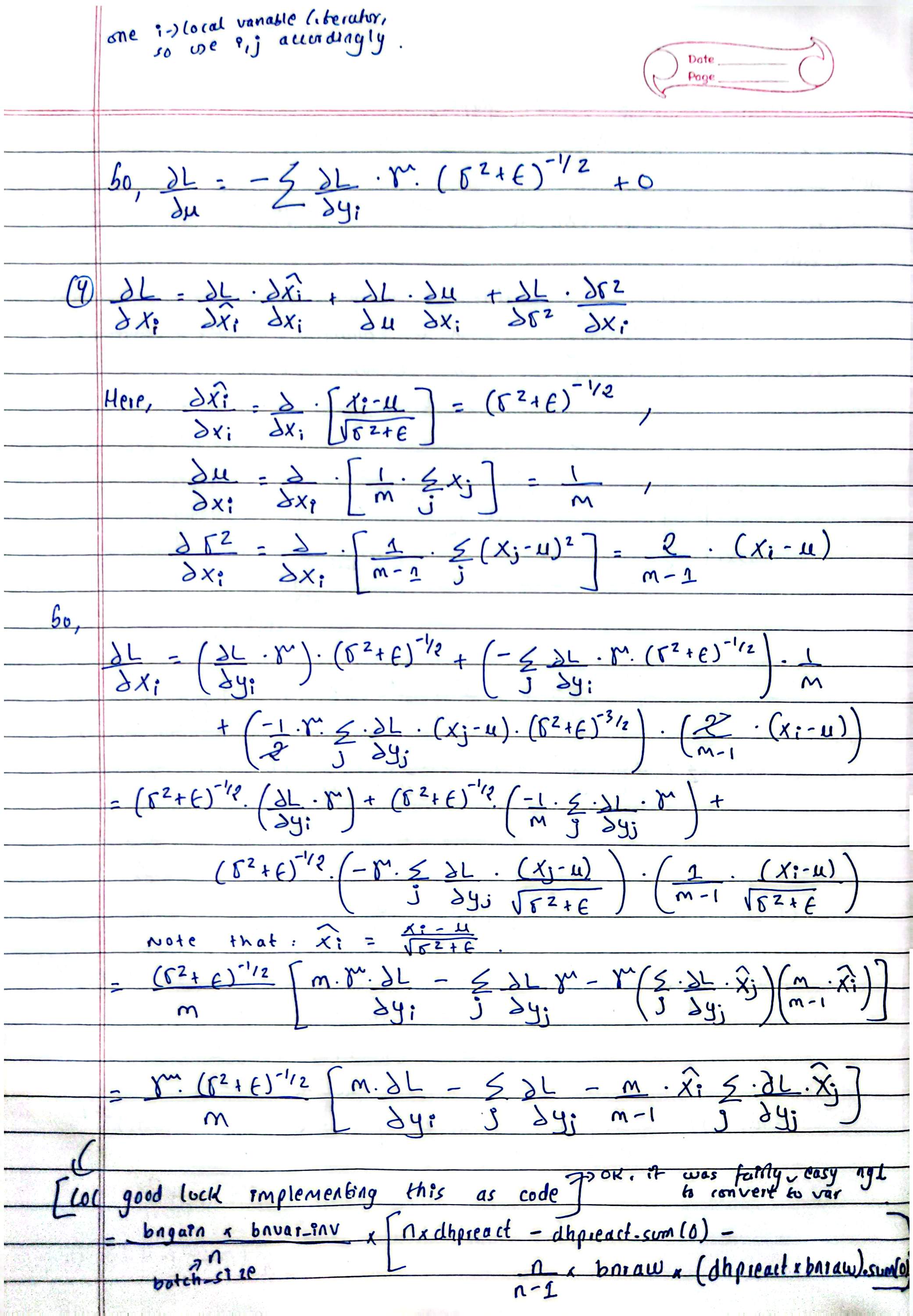
# in the batchnorm paper, hprebn is x and hpreact is y
# in the backward pass we have dhpreact, and we'd like to produce dhprebn
# Exercise 3: backprop through batchnorm but all in one go
# to complete this challenge look at the mathematical expression of the output of batchnorm,
# take the derivative w.r.t. its input, simplify the expression, and just write it out
# forward pass
# before:
# bnmeani = 1/n*hprebn.sum(0, keepdim=True)
# bndiff = hprebn - bnmeani
# bndiff2 = bndiff**2
# bnvar = 1/(n-1)*(bndiff2).sum(0, keepdim=True) # note: Bessel's correction (dividing by n-1, not n)
# bnvar_inv = (bnvar + 1e-5)**-0.5
# bnraw = bndiff * bnvar_inv
# hpreact = bngain * bnraw + bnbias
# now:
# hpreact_fast = bngain * (hprebn - hprebn.mean(0, keepdim=True)) / torch.sqrt(hprebn.var(0, keepdim=True, unbiased=True) + 1e-5) + bnbias
# print('max diff:', (hpreact_fast - hpreact).abs().max())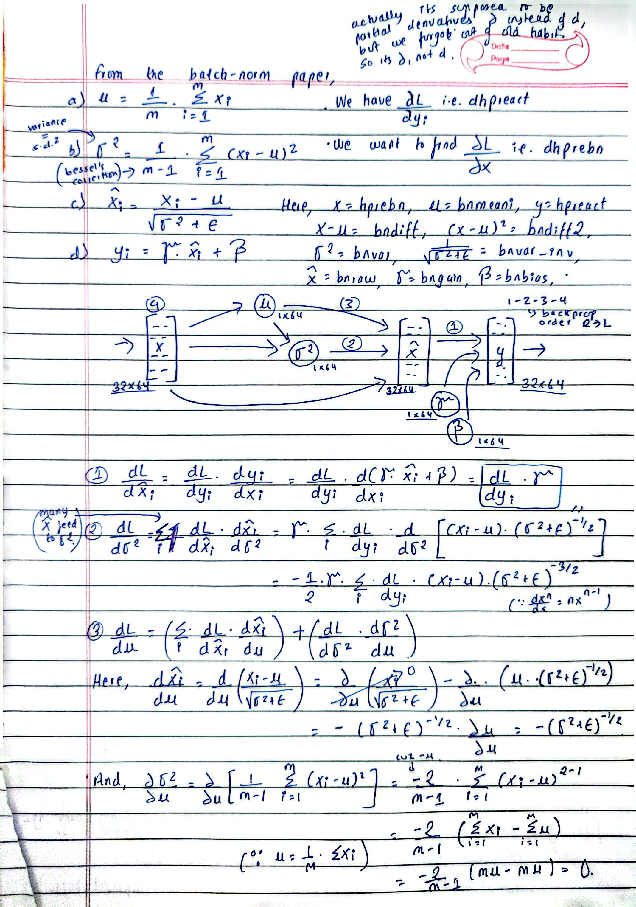
# # backward pass

# # before we had:
# # dbnraw = bngain * dhpreact
# # dbndiff = bnvar_inv * dbnraw
# # dbnvar_inv = (bndiff * dbnraw).sum(0, keepdim=True)
# # dbnvar = (-0.5*(bnvar + 1e-5)**-1.5) * dbnvar_inv
# # dbndiff2 = (1.0/(n-1))*torch.ones_like(bndiff2) * dbnvar
# # dbndiff += (2*bndiff) * dbndiff2
# # dhprebn = dbndiff.clone()
# # dbnmeani = (-dbndiff).sum(0)
# # dhprebn += 1.0/n * (torch.ones_like(hprebn) * dbnmeani)

# # calculate dhprebn given dhpreact (i.e. backprop through the batchnorm)
# # (you'll also need to use some of the variables from the forward pass up above)

dhprebn = bngain*bnvar_inv/n * (n*dhpreact - dhpreact.sum(0) - n/(n-1)*bnraw*(dhpreact*bnraw).sum(0))
cmp('hprebn', dhprebn, hprebn) # I can only get approximate to be true, my maxdiff is 9e-10
# print(hprebn.shape, bnmeani.shape, bnvar.shape, bnraw.shape, bngain.shape, bnbias.shape, hpreact.shape)
hprebn | exact: False | approximate: True | maxdiff: 9.313225746154785e-10
# dhprebn.shape, bngain.shape, bnvar_inv.shape, dbnraw.shape, dbnraw.sum(0).shapeTraining with the manual backward pass
# Exercise 4: putting it all together!
# Train the MLP neural net with your own backward pass

# init
n_embd = 10 # the dimensionality of the character embedding vectors
n_hidden = 200 # the number of neurons in the hidden layer of the MLP

g = torch.Generator().manual_seed(2147483647) # for reproducibility
C  = torch.randn((vocab_size, n_embd),            generator=g)
# Layer 1
W1 = torch.randn((n_embd * block_size, n_hidden), generator=g) * (5/3)/((n_embd * block_size)**0.5)
b1 = torch.randn(n_hidden,                        generator=g) * 0.1
# Layer 2
W2 = torch.randn((n_hidden, vocab_size),          generator=g) * 0.1
b2 = torch.randn(vocab_size,                      generator=g) * 0.1
# BatchNorm parameters
bngain = torch.randn((1, n_hidden))*0.1 + 1.0
bnbias = torch.randn((1, n_hidden))*0.1

parameters = [C, W1, b1, W2, b2, bngain, bnbias]
print(sum(p.nelement() for p in parameters)) # number of parameters in total
for p in parameters:
  p.requires_grad = True

# same optimization as last time
max_steps = 200000
batch_size = 32
n = batch_size # convenience
lossi = []

# use this context manager for efficiency once your backward pass is written (TODO)
with torch.no_grad():

  # kick off optimization
  for i in range(max_steps):

    # minibatch construct
    ix = torch.randint(0, Xtr.shape[0], (batch_size,), generator=g)
    Xb, Yb = Xtr[ix], Ytr[ix] # batch X,Y

    # forward pass
    emb = C[Xb] # embed the characters into vectors
    embcat = emb.view(emb.shape[0], -1) # concatenate the vectors
    # Linear layer
    hprebn = embcat @ W1 + b1 # hidden layer pre-activation
    # BatchNorm layer
    # -------------------------------------------------------------
    bnmean = hprebn.mean(0, keepdim=True)
    bnvar = hprebn.var(0, keepdim=True, unbiased=True)
    bnvar_inv = (bnvar + 1e-5)**-0.5
    bnraw = (hprebn - bnmean) * bnvar_inv
    hpreact = bngain * bnraw + bnbias
    # -------------------------------------------------------------
    # Non-linearity
    h = torch.tanh(hpreact) # hidden layer
    logits = h @ W2 + b2 # output layer
    loss = F.cross_entropy(logits, Yb) # loss function

    # backward pass
    for p in parameters:
      p.grad = None
    #loss.backward() # use this for correctness comparisons, delete it later!

    # manual backprop!
    # -----------------
    dlogits = F.softmax(logits, 1)
    dlogits[range(n), Yb] -= 1
    dlogits /= n
    # 2nd layer backprop
    dh = dlogits @ W2.T
    dW2 = h.T @ dlogits
    db2 = dlogits.sum(0)
    # tanh
    dhpreact = (1.0 - h**2) * dh
    # batchnorm backprop
    dbngain = (bnraw * dhpreact).sum(0, keepdim=True)
    dbnbias = dhpreact.sum(0, keepdim=True)
    dhprebn = bngain*bnvar_inv/n * (n*dhpreact - dhpreact.sum(0) - n/(n-1)*bnraw*(dhpreact*bnraw).sum(0))
    # 1st layer
    dembcat = dhprebn @ W1.T
    dW1 = embcat.T @ dhprebn
    db1 = dhprebn.sum(0)
    # embedding
    demb = dembcat.view(emb.shape)
    dC = torch.zeros_like(C)
    for k in range(Xb.shape[0]):
      for j in range(Xb.shape[1]):
        ix = Xb[k,j]
        dC[ix] += demb[k,j]
    grads = [dC, dW1, db1, dW2, db2, dbngain, dbnbias]
    # -----------------

    # update
    lr = 0.1 if i < 100000 else 0.01 # step learning rate decay
    for p, grad in zip(parameters, grads):
      #p.data += -lr * p.grad # old way (using PyTorch grad from .backward())
      p.data += -lr * grad # new way

    # track stats
    if i % 10000 == 0: # print every once in a while
      print(f'{i:7d}/{max_steps:7d}: {loss.item():.4f}')
    lossi.append(loss.log10().item())

  #   if i >= 100: # TODO: delete early breaking when you're ready to train the full net
  #     break
12297
0/ 200000: 3.7948
10000/ 200000: 2.1612
20000/ 200000: 2.3483
30000/ 200000: 2.4187
40000/ 200000: 1.9691
50000/ 200000: 2.3682
60000/ 200000: 2.3674
70000/ 200000: 2.0210
80000/ 200000: 2.3817
90000/ 200000: 2.0875
100000/ 200000: 2.0010
110000/ 200000: 2.4035
120000/ 200000: 2.0293
---------------------------------------------------------------------------
KeyboardInterrupt                         Traceback (most recent call last)
Cell In[82], line 82
     78     dhprebn = bngain*bnvar_inv/n * (n*dhpreact - dhpreact.sum(0) - n/(n-1)*bnraw*(dhpreact*bnraw).sum(0))
     79     # 1st layer
     80     dembcat = dhprebn @ W1.T
     81     dW1 = embcat.T @ dhprebn
---> 82     db1 = dhprebn.sum(0)
     83     # embedding
     84     demb = dembcat.view(emb.shape)
     85     dC = torch.zeros_like(C)

KeyboardInterrupt:
# # useful for checking your gradients
# for p,g in zip(parameters, grads):
# cmp(str(tuple(p.shape)), g, p)# calibrate the batch norm at the end of training
with torch.no_grad():
# pass the training set through
emb = C[Xtr]
embcat = emb.view(emb.shape[0], -1)
hpreact = embcat @ W1 + b1
# measure the mean/std over the entire training set
bnmean = hpreact.mean(0, keepdim=True)
bnvar = hpreact.var(0, keepdim=True, unbiased=True)
# evaluate train and val loss

@torch.no_grad() # this decorator disables gradient tracking
def split_loss(split):
  x,y = {
    'train': (Xtr, Ytr),
    'val': (Xdev, Ydev),
    'test': (Xte, Yte),
  }[split]
  emb = C[x] # (N, block_size, n_embd)
  embcat = emb.view(emb.shape[0], -1) # concat into (N, block_size * n_embd)
  hpreact = embcat @ W1 + b1
  hpreact = bngain * (hpreact - bnmean) * (bnvar + 1e-5)**-0.5 + bnbias
  h = torch.tanh(hpreact) # (N, n_hidden)
  logits = h @ W2 + b2 # (N, vocab_size)
  loss = F.cross_entropy(logits, y)
  print(split, loss.item())

split_loss('train')
split_loss('val')
train 2.079331398010254
val 2.115342855453491
# Andrej achieved:
# train 2.0718822479248047
# val 2.1162495613098145
# I achieved:
# train 2.079331398010254
# val 2.115342855453491# sample from the model
g = torch.Generator().manual_seed(2147483647 + 10)
for _ in range(20):
out = []
context = [0] * block_size # initialize with all ...
while True:
# ------------
# forward pass:
# Embedding
emb = C[torch.tensor([context])] # (1,block_size,d)
embcat = emb.view(emb.shape[0], -1) # concat into (N, block_size * n_embd)
hpreact = embcat @ W1 + b1
hpreact = bngain * (hpreact - bnmean) * (bnvar + 1e-5)**-0.5 + bnbias
h = torch.tanh(hpreact) # (N, n_hidden)
logits = h @ W2 + b2 # (N, vocab_size)
# ------------
# Sample
probs = F.softmax(logits, dim=1)
ix = torch.multinomial(probs, num_samples=1, generator=g).item()
context = context[1:] + [ix]
out.append(ix)
if ix == 0:
break
print(''.join(itos[i] for i in out))carmah.
amelle.
khi.
mri.
reity.
salayson.
rahnen.
delynn.
jarqui.
nellara.
chaiivon.
leigh.
ham.
joce.
quint.
sulio.
alianni.
waverogiearynix.
kael.
dura.