Bigram language models
Original study notes by Satish Bajagain, following Andrej Karpathy’s Zero to Hero. Comments, intermediate attempts and saved outputs are retained. Section titles are navigation additions.
Characters and bigrams
# makemore is a character-level language model
# so it models the given sequence of characters, e.g. one example is given as: alyssa, there are 32k such examples
# then it can predict the next character in the sequence
# we will go from character-level(bigram), to word-level(bag of words), mlp, rnn, gru, finally modern transformers(on which gpt-2 is based on)# first, let's load up the dataset "names.txt"
# open("names.txt", "r").readlines()[5:20]
# .read(5) reads the first 5 characters, not the first 5 namesopen("names.txt", "r").read()#read everything into a massive string
# since it's a massive string, we only want the individual words, and put them in a list
words = open("names.txt", "r").read().splitlines()
words[:20]#look at first 20 words['emma',
'olivia',
'ava',
'isabella',
'sophia',
'charlotte',
'mia',
'amelia',
'harper',
'evelyn',
'abigail',
'emily',
'elizabeth',
'mila',
'ella',
'avery',
'sofia',
'camila',
'aria',
'scarlett']# let's learn more about this dataset, let's look at the total number of words
len(words)32033# let's find the shortest word
print(min(len(w) for w in words))
print(min(words, key=len))2
an
# longest word
print(max(len(w) for w in words))
print(max(words, key=len))
15
muhammadibrahim
# a character level language model is predicting the next character in a sequence given already some concrete sequence of characters before it
# for eg. if there is a word named isabella, it says that the character 'i' is very likely to occur first in the new name
# the character 's' is likely to come after i
# the character 'a' is likely to come after is, and so on
# and the last piece of information: after the sequence becomes 'isabella', the word is likely to end
# in a bigram language model, we are always working with only 2 characters at a time
# we are looking only at the one character we are given, and are trying to predict the next character in the sequence
# eg. what characters are likely to follow 'r', or likely to follow 'a', and so on.
# we are just modeling this little structure
# atleast for now, we are ignoring the fact that we have more information through the entire word
# HERE: WE ARE JUST LOOKING AT THE PREVIOUS CHARACTER TO PREDICT THE NEXT ONE
# and this is a very simple and weak language model# now, let's look at what bigrams in our dataset look like
# bigrams: just 2 characters in a rowprint(words[0])
print(words[:1])emma
['emma']
# we want 2 characters at a time sliding through the entire word
for w in words[:1]:
    for ch1, ch2 in zip(w, w[1:]):
        print(ch1, ch2)
e m
m m
m a
# continue from 8:14
# so, e is likely to come first, and a is likely to come last
# we are going to create a special array of characters, and we're going to hallucinate a special start token here, then the word, then the special endfor w in words[:1]:
chs = ['<S>'] + list(w) + ['<E>']
for ch1, ch2 in zip(chs, chs[1:]):
print(ch1, ch2)<S> e
e m
m m
m a
a <E>
for w in words[:3]:
    chs = ['<S>'] + list(w) + ['<E>']
    for ch1, ch2 in zip(chs, chs[1:]):
        print(ch1, ch2)
<S> e
e m
m m
m a
a <E>
<S> o
o l
l i
i v
v i
i a
a <E>
<S> a
a v
v a
a <E>
# TO LEARN THE STATISTICS ABOUT WHICH CHARACTERS ARE MORE LIKELY TO FOLLOW OTHER CHARACTERS,
# THE SIMPLEST WAY IN THE BIGRAM LANGUAGE MODELS IS TO SIMPLY DO IT BY COUNTING
# SO WE'RE JUST GOING TO COUNT HOW OFTEN ANY ONE OF THESE COMBINATIONS OCCURS IN THE TRAINING SET
# so we need a dictionary to maintain some counts for every one of these bigrams, let's use a dictionary b
# bigram is a tuple of character 1, character 2
b = {}
for w in words[:3]:
chs = ['<S>'] + list(w) + ['<E>']
for ch1, ch2 in zip(chs, chs[1:]):
bigram = (ch1, ch2)
b[bigram] = b.get(bigram, 0) + 1
# in the case that bigram is not in dictionary b, we would like to return 0 by default
# the +1 will add up all bigrams and count how often they occur
print(ch1, ch2)<S> e
e m
m m
m a
a <E>
<S> o
o l
l i
i v
v i
i a
a <E>
<S> a
a v
v a
a <E>
b{('<S>', 'e'): 1,
('e', 'm'): 1,
('m', 'm'): 1,
('m', 'a'): 1,
('a', '<E>'): 3,
('<S>', 'o'): 1,
('o', 'l'): 1,
('l', 'i'): 1,
('i', 'v'): 1,
('v', 'i'): 1,
('i', 'a'): 1,
('<S>', 'a'): 1,
('a', 'v'): 1,
('v', 'a'): 1}# note that for these 3 words, a was always the ending character everytime so the count is 3 which is what we want to see# now let's maintain count of bigrams for all the words instead
b = {}
for w in words:
chs = ['<S>'] + list(w) + ['<E>']
for ch1, ch2 in zip(chs, chs[1:]):
bigram = (ch1, ch2)
b[bigram] = b.get(bigram, 0) + 1b{('<S>', 'e'): 1531,
('e', 'm'): 769,
('m', 'm'): 168,
('m', 'a'): 2590,
('a', '<E>'): 6640,
('<S>', 'o'): 394,
('o', 'l'): 619,
('l', 'i'): 2480,
('i', 'v'): 269,
('v', 'i'): 911,
('i', 'a'): 2445,
('<S>', 'a'): 4410,
('a', 'v'): 834,
('v', 'a'): 642,
('<S>', 'i'): 591,
('i', 's'): 1316,
('s', 'a'): 1201,
('a', 'b'): 541,
('b', 'e'): 655,
('e', 'l'): 3248,
('l', 'l'): 1345,
('l', 'a'): 2623,
('<S>', 's'): 2055,
('s', 'o'): 531,
('o', 'p'): 95,
('p', 'h'): 204,
('h', 'i'): 729,
('<S>', 'c'): 1542,
('c', 'h'): 664,
('h', 'a'): 2244,
('a', 'r'): 3264,
('r', 'l'): 413,
('l', 'o'): 692,
('o', 't'): 118,
('t', 't'): 374,
('t', 'e'): 716,
('e', '<E>'): 3983,
('<S>', 'm'): 2538,
('m', 'i'): 1256,
('a', 'm'): 1634,
('m', 'e'): 818,
('<S>', 'h'): 874,
('r', 'p'): 14,
('p', 'e'): 197,
('e', 'r'): 1958,
('r', '<E>'): 1377,
('e', 'v'): 463,
('v', 'e'): 568,
('l', 'y'): 1588,
('y', 'n'): 1826,
('n', '<E>'): 6763,
('b', 'i'): 217,
('i', 'g'): 428,
('g', 'a'): 330,
('a', 'i'): 1650,
('i', 'l'): 1345,
('l', '<E>'): 1314,
('y', '<E>'): 2007,
('i', 'z'): 277,
('z', 'a'): 860,
('e', 't'): 580,
('t', 'h'): 647,
('h', '<E>'): 2409,
('r', 'y'): 773,
('o', 'f'): 34,
('f', 'i'): 160,
('c', 'a'): 815,
('r', 'i'): 3033,
('s', 'c'): 60,
('l', 'e'): 2921,
('t', '<E>'): 483,
('<S>', 'v'): 376,
('i', 'c'): 509,
('c', 't'): 35,
('t', 'o'): 667,
('o', 'r'): 1059,
('a', 'd'): 1042,
('d', 'i'): 674,
('o', 'n'): 2411,
('<S>', 'l'): 1572,
('l', 'u'): 324,
('u', 'n'): 275,
('n', 'a'): 2977,
('<S>', 'g'): 669,
('g', 'r'): 201,
('r', 'a'): 2356,
('a', 'c'): 470,
('c', 'e'): 551,
('h', 'l'): 185,
('o', 'e'): 132,
('<S>', 'p'): 515,
('e', 'n'): 2675,
('n', 'e'): 1359,
('a', 'y'): 2050,
('y', 'l'): 1104,
('<S>', 'r'): 1639,
('e', 'y'): 1070,
('<S>', 'z'): 929,
('z', 'o'): 110,
('<S>', 'n'): 1146,
('n', 'o'): 496,
('e', 'a'): 679,
('a', 'n'): 5438,
('n', 'n'): 1906,
('a', 'h'): 2332,
('d', 'd'): 149,
('a', 'u'): 381,
('u', 'b'): 103,
('b', 'r'): 842,
('r', 'e'): 1697,
('i', 'e'): 1653,
('s', 't'): 765,
('a', 't'): 687,
('t', 'a'): 1027,
('a', 'l'): 2528,
('a', 'z'): 435,
('z', 'e'): 373,
('i', 'o'): 588,
('u', 'r'): 414,
('r', 'o'): 869,
('u', 'd'): 136,
('d', 'r'): 424,
('<S>', 'b'): 1306,
('o', 'o'): 115,
('o', 'k'): 68,
('k', 'l'): 139,
('c', 'l'): 116,
('i', 'r'): 849,
('s', 'k'): 82,
('k', 'y'): 379,
('u', 'c'): 103,
('c', 'y'): 104,
('p', 'a'): 209,
('s', 'l'): 279,
('i', 'n'): 2126,
('o', 'v'): 176,
('g', 'e'): 334,
('e', 's'): 861,
('s', 'i'): 684,
('s', '<E>'): 1169,
('<S>', 'k'): 2963,
('k', 'e'): 895,
('e', 'd'): 384,
('d', 'y'): 317,
('n', 't'): 443,
('y', 'a'): 2143,
('<S>', 'w'): 307,
('w', 'i'): 148,
('o', 'w'): 114,
('w', '<E>'): 51,
('k', 'i'): 509,
('n', 's'): 278,
('a', 'o'): 63,
('o', 'm'): 261,
('i', '<E>'): 2489,
('a', 'a'): 556,
('i', 'y'): 779,
('d', 'e'): 1283,
('c', 'o'): 380,
('r', 'u'): 252,
('b', 'y'): 83,
('s', 'e'): 884,
('n', 'i'): 1725,
('i', 't'): 541,
('t', 'y'): 341,
('u', 't'): 82,
('t', 'u'): 78,
('u', 'm'): 154,
('m', 'n'): 20,
('g', 'i'): 190,
('t', 'i'): 532,
('<S>', 'q'): 92,
('q', 'u'): 206,
('u', 'i'): 121,
('a', 'e'): 692,
('e', 'h'): 152,
('v', 'y'): 121,
('p', 'i'): 61,
('i', 'p'): 53,
('y', 'd'): 272,
('e', 'x'): 132,
('x', 'a'): 103,
('<S>', 'j'): 2422,
('j', 'o'): 479,
('o', 's'): 504,
('e', 'p'): 83,
('j', 'u'): 202,
('u', 'l'): 301,
('<S>', 'd'): 1690,
('k', 'a'): 1731,
('e', 'e'): 1271,
('y', 't'): 104,
('d', 'l'): 60,
('c', 'k'): 316,
('n', 'z'): 145,
('z', 'i'): 364,
('a', 'g'): 168,
('d', 'a'): 1303,
('j', 'a'): 1473,
('h', 'e'): 674,
('<S>', 'x'): 134,
('x', 'i'): 102,
('i', 'm'): 427,
('e', 'i'): 818,
('<S>', 't'): 1308,
('<S>', 'f'): 417,
('f', 'a'): 242,
('n', 'd'): 704,
('r', 'g'): 76,
('a', 's'): 1118,
('s', 'h'): 1285,
('b', 'a'): 321,
('k', 'h'): 307,
('s', 'm'): 90,
('o', 'd'): 190,
('r', 's'): 190,
('g', 'h'): 360,
('s', 'y'): 215,
('y', 's'): 401,
('s', 's'): 461,
('e', 'c'): 153,
('c', 'i'): 271,
('m', 'o'): 452,
('r', 'k'): 90,
('n', 'l'): 195,
('d', 'n'): 31,
('r', 'd'): 187,
('o', 'i'): 69,
('t', 'r'): 352,
('m', 'b'): 112,
('r', 'm'): 162,
('n', 'y'): 465,
('d', 'o'): 378,
('o', 'a'): 149,
('o', 'c'): 114,
('m', 'y'): 287,
('s', 'u'): 185,
('m', 'c'): 51,
('p', 'r'): 151,
('o', 'u'): 275,
('r', 'n'): 140,
('w', 'a'): 280,
('e', 'b'): 121,
('c', 'c'): 42,
('a', 'w'): 161,
('w', 'y'): 73,
('y', 'e'): 301,
('e', 'o'): 269,
('a', 'k'): 568,
('n', 'g'): 273,
('k', 'o'): 344,
('b', 'l'): 103,
('h', 'o'): 287,
('e', 'g'): 125,
('f', 'r'): 114,
('s', 'p'): 51,
('l', 's'): 94,
('y', 'z'): 78,
('g', 'g'): 25,
('z', 'u'): 73,
('i', 'd'): 440,
('m', '<E>'): 516,
('o', 'g'): 44,
('j', 'e'): 440,
('g', 'n'): 27,
('y', 'r'): 291,
('c', '<E>'): 97,
('c', 'q'): 11,
('u', 'e'): 169,
('i', 'f'): 101,
('f', 'e'): 123,
('i', 'x'): 89,
('x', '<E>'): 164,
('o', 'y'): 103,
('g', 'o'): 83,
('g', 't'): 31,
('l', 't'): 77,
('g', 'w'): 26,
('w', 'e'): 149,
('l', 'd'): 138,
('a', 'p'): 82,
('h', 'n'): 138,
('t', 'l'): 134,
('m', 'r'): 97,
('n', 'c'): 213,
('l', 'b'): 52,
('i', 'k'): 445,
('<S>', 'y'): 535,
('t', 'z'): 105,
('h', 'r'): 204,
('j', 'i'): 119,
('h', 't'): 71,
('r', 'r'): 425,
('z', 'l'): 123,
('w', 'r'): 22,
('b', 'b'): 38,
('r', 't'): 208,
('l', 'v'): 72,
('e', 'j'): 55,
('o', 'h'): 171,
('u', 's'): 474,
('i', 'b'): 110,
('g', 'l'): 32,
('h', 'y'): 213,
('p', 'o'): 59,
('p', 'p'): 39,
('p', 'y'): 12,
('n', 'r'): 44,
('z', 'm'): 35,
('v', 'o'): 153,
('l', 'm'): 60,
('o', 'x'): 45,
('d', '<E>'): 516,
('i', 'u'): 109,
('v', '<E>'): 88,
('f', 'f'): 44,
('b', 'o'): 105,
('e', 'k'): 178,
('c', 'r'): 76,
('d', 'g'): 25,
('r', 'c'): 99,
('r', 'h'): 121,
('n', 'k'): 58,
('h', 'u'): 166,
('d', 's'): 29,
('a', 'x'): 182,
('y', 'c'): 115,
('e', 'w'): 50,
('v', 'k'): 3,
('z', 'h'): 43,
('w', 'h'): 23,
('t', 'n'): 22,
('x', 'l'): 39,
('g', 'u'): 85,
('u', 'a'): 163,
('u', 'p'): 16,
('u', 'g'): 47,
('d', 'u'): 92,
('l', 'c'): 25,
('r', 'b'): 41,
('a', 'q'): 60,
('b', '<E>'): 114,
('g', 'y'): 31,
('y', 'p'): 15,
('p', 't'): 17,
('e', 'z'): 181,
('z', 'r'): 32,
('f', 'l'): 20,
('o', '<E>'): 855,
('o', 'b'): 140,
('u', 'z'): 45,
('z', '<E>'): 160,
('i', 'q'): 52,
('y', 'v'): 106,
('n', 'v'): 55,
('d', 'h'): 118,
('g', 'd'): 19,
('t', 's'): 35,
('n', 'h'): 26,
('y', 'j'): 23,
('k', 'r'): 109,
('z', 'b'): 4,
('g', '<E>'): 108,
('a', 'j'): 175,
('r', 'j'): 25,
('m', 'p'): 38,
('p', 'b'): 2,
('y', 'o'): 271,
('z', 'y'): 147,
('p', 'l'): 16,
('l', 'k'): 24,
('i', 'j'): 76,
('x', 'e'): 36,
('y', 'u'): 141,
('l', 'n'): 14,
('u', 'x'): 34,
('i', 'h'): 95,
('w', 's'): 20,
('k', 's'): 95,
('m', 'u'): 139,
('y', 'k'): 86,
('e', 'f'): 82,
('k', '<E>'): 363,
('y', 'm'): 148,
('z', 'z'): 45,
('m', 'd'): 24,
('s', 'r'): 55,
('e', 'u'): 69,
('l', 'h'): 19,
('a', 'f'): 134,
('r', 'w'): 21,
('n', 'u'): 96,
('v', 'r'): 48,
('m', 's'): 35,
('<S>', 'u'): 78,
('f', 's'): 6,
('y', 'b'): 27,
('x', 'o'): 41,
('g', 's'): 30,
('x', 'y'): 30,
('w', 'n'): 58,
('j', 'h'): 45,
('f', 'n'): 4,
('n', 'j'): 44,
('r', 'v'): 80,
('n', 'm'): 19,
('t', 'c'): 17,
('s', 'w'): 24,
('k', 't'): 17,
('f', 't'): 18,
('x', 't'): 70,
('u', 'v'): 37,
('k', 'k'): 20,
('s', 'n'): 24,
('u', '<E>'): 155,
('j', 'r'): 11,
('y', 'x'): 28,
('h', 'm'): 117,
('e', 'q'): 14,
('u', 'o'): 10,
('f', '<E>'): 80,
('h', 'z'): 20,
('h', 'k'): 29,
('y', 'g'): 30,
('q', 'r'): 1,
('v', 'n'): 8,
('s', 'd'): 9,
('y', 'i'): 192,
('n', 'w'): 11,
('d', 'v'): 17,
('h', 'v'): 39,
('x', 'w'): 3,
('o', 'z'): 54,
('k', 'u'): 50,
('u', 'h'): 58,
('k', 'n'): 26,
('s', 'b'): 21,
('i', 'i'): 82,
('y', 'y'): 23,
('r', 'z'): 23,
('l', 'g'): 6,
('l', 'p'): 15,
('p', '<E>'): 33,
('b', 'u'): 45,
('f', 'u'): 10,
('b', 'h'): 41,
('f', 'y'): 14,
('u', 'w'): 86,
('x', 'u'): 5,
('q', '<E>'): 28,
('l', 'r'): 18,
('m', 'h'): 5,
('l', 'w'): 16,
('j', '<E>'): 71,
('s', 'v'): 14,
('m', 'l'): 5,
('n', 'f'): 11,
('u', 'j'): 14,
('f', 'o'): 60,
('j', 'l'): 9,
('t', 'g'): 2,
('j', 'm'): 5,
('v', 'v'): 7,
('p', 's'): 16,
('t', 'w'): 11,
('x', 'c'): 4,
('u', 'k'): 93,
('v', 'l'): 14,
('h', 'd'): 24,
('l', 'z'): 10,
('k', 'w'): 34,
('n', 'b'): 8,
('q', 's'): 2,
('i', 'w'): 8,
('c', 's'): 5,
('h', 's'): 31,
('m', 't'): 4,
('h', 'w'): 10,
('x', 'x'): 38,
('t', 'x'): 2,
('d', 'z'): 1,
('x', 'z'): 19,
('t', 'm'): 4,
('t', 'j'): 3,
('u', 'q'): 10,
('q', 'a'): 13,
('f', 'k'): 2,
('z', 'n'): 4,
('l', 'j'): 6,
('j', 'w'): 6,
('v', 'u'): 7,
('c', 'j'): 3,
('h', 'b'): 8,
('z', 't'): 4,
('p', 'u'): 4,
('m', 'z'): 11,
('x', 's'): 31,
('b', 't'): 2,
('u', 'y'): 13,
('d', 'j'): 9,
('j', 's'): 7,
('w', 'u'): 25,
('o', 'j'): 16,
('b', 's'): 8,
('d', 'w'): 23,
('w', 'o'): 36,
('j', 'n'): 2,
('w', 't'): 8,
('l', 'f'): 22,
('d', 'm'): 30,
('p', 'j'): 1,
('j', 'y'): 10,
('y', 'f'): 12,
('q', 'i'): 13,
('j', 'v'): 5,
('q', 'l'): 1,
('s', 'z'): 10,
('k', 'm'): 9,
('w', 'l'): 13,
('p', 'f'): 1,
('q', 'w'): 3,
('n', 'x'): 6,
('k', 'c'): 2,
('t', 'v'): 15,
('c', 'u'): 35,
('z', 'k'): 2,
('c', 'z'): 4,
('y', 'q'): 6,
('y', 'h'): 22,
('r', 'f'): 9,
('s', 'j'): 2,
('h', 'j'): 9,
('g', 'b'): 3,
('u', 'f'): 19,
('s', 'f'): 2,
('q', 'e'): 1,
('b', 'c'): 1,
('c', 'd'): 1,
('z', 'j'): 2,
('n', 'q'): 2,
('m', 'f'): 1,
('p', 'n'): 1,
('f', 'z'): 2,
('b', 'n'): 4,
('w', 'd'): 8,
('w', 'b'): 1,
('b', 'd'): 65,
('z', 's'): 4,
('p', 'c'): 1,
('h', 'g'): 2,
('m', 'j'): 7,
('w', 'w'): 2,
('k', 'j'): 2,
('h', 'p'): 1,
('j', 'k'): 2,
('o', 'q'): 3,
('f', 'w'): 4,
('f', 'h'): 1,
('w', 'm'): 2,
('b', 'j'): 1,
('r', 'q'): 16,
('z', 'c'): 2,
('z', 'v'): 2,
('f', 'g'): 1,
('n', 'p'): 5,
('z', 'g'): 1,
('d', 't'): 4,
('w', 'f'): 2,
('d', 'f'): 5,
('w', 'k'): 6,
('q', 'm'): 2,
('k', 'z'): 2,
('j', 'j'): 2,
('c', 'p'): 1,
('p', 'k'): 1,
('p', 'm'): 1,
('j', 'd'): 4,
('r', 'x'): 3,
('x', 'n'): 1,
('d', 'c'): 3,
('g', 'j'): 3,
('x', 'f'): 3,
('j', 'c'): 4,
('s', 'q'): 1,
('k', 'f'): 1,
('z', 'p'): 2,
('j', 't'): 2,
('k', 'b'): 2,
('m', 'k'): 1,
('m', 'w'): 2,
('x', 'h'): 1,
('h', 'f'): 2,
('x', 'd'): 5,
('y', 'w'): 4,
('z', 'w'): 3,
('d', 'k'): 3,
('c', 'g'): 2,
('u', 'u'): 3,
('t', 'f'): 2,
('g', 'm'): 6,
('m', 'v'): 3,
('c', 'x'): 3,
('h', 'c'): 2,
('g', 'f'): 1,
('q', 'o'): 2,
('l', 'q'): 3,
('v', 'b'): 1,
('j', 'p'): 1,
('k', 'd'): 2,
('g', 'z'): 1,
('v', 'd'): 1,
('d', 'b'): 1,
('v', 'h'): 1,
('k', 'v'): 2,
('h', 'h'): 1,
('s', 'g'): 2,
('g', 'v'): 1,
('d', 'q'): 1,
('x', 'b'): 1,
('w', 'z'): 1,
('h', 'q'): 1,
('j', 'b'): 1,
('z', 'd'): 2,
('x', 'm'): 1,
('w', 'g'): 1,
('t', 'b'): 1,
('z', 'x'): 1}# b.items() returns the tuples of key-value
# in this case, the keys are character bigrams and values are the counts
# we want to sort, but the default sort is on the first item of the tuple, but we want to sort by count here which is the second element of the tuple
# so we added key = lambda that takes the key value and returns keyvalue at [1] instead of default [0]
# and we want to do it in descending order by using -ve signb.items()dict_items([(('<S>', 'e'), 1531), (('e', 'm'), 769), (('m', 'm'), 168), (('m', 'a'), 2590), (('a', '<E>'), 6640), (('<S>', 'o'), 394), (('o', 'l'), 619), (('l', 'i'), 2480), (('i', 'v'), 269), (('v', 'i'), 911), (('i', 'a'), 2445), (('<S>', 'a'), 4410), (('a', 'v'), 834), (('v', 'a'), 642), (('<S>', 'i'), 591), (('i', 's'), 1316), (('s', 'a'), 1201), (('a', 'b'), 541), (('b', 'e'), 655), (('e', 'l'), 3248), (('l', 'l'), 1345), (('l', 'a'), 2623), (('<S>', 's'), 2055), (('s', 'o'), 531), (('o', 'p'), 95), (('p', 'h'), 204), (('h', 'i'), 729), (('<S>', 'c'), 1542), (('c', 'h'), 664), (('h', 'a'), 2244), (('a', 'r'), 3264), (('r', 'l'), 413), (('l', 'o'), 692), (('o', 't'), 118), (('t', 't'), 374), (('t', 'e'), 716), (('e', '<E>'), 3983), (('<S>', 'm'), 2538), (('m', 'i'), 1256), (('a', 'm'), 1634), (('m', 'e'), 818), (('<S>', 'h'), 874), (('r', 'p'), 14), (('p', 'e'), 197), (('e', 'r'), 1958), (('r', '<E>'), 1377), (('e', 'v'), 463), (('v', 'e'), 568), (('l', 'y'), 1588), (('y', 'n'), 1826), (('n', '<E>'), 6763), (('b', 'i'), 217), (('i', 'g'), 428), (('g', 'a'), 330), (('a', 'i'), 1650), (('i', 'l'), 1345), (('l', '<E>'), 1314), (('y', '<E>'), 2007), (('i', 'z'), 277), (('z', 'a'), 860), (('e', 't'), 580), (('t', 'h'), 647), (('h', '<E>'), 2409), (('r', 'y'), 773), (('o', 'f'), 34), (('f', 'i'), 160), (('c', 'a'), 815), (('r', 'i'), 3033), (('s', 'c'), 60), (('l', 'e'), 2921), (('t', '<E>'), 483), (('<S>', 'v'), 376), (('i', 'c'), 509), (('c', 't'), 35), (('t', 'o'), 667), (('o', 'r'), 1059), (('a', 'd'), 1042), (('d', 'i'), 674), (('o', 'n'), 2411), (('<S>', 'l'), 1572), (('l', 'u'), 324), (('u', 'n'), 275), (('n', 'a'), 2977), (('<S>', 'g'), 669), (('g', 'r'), 201), (('r', 'a'), 2356), (('a', 'c'), 470), (('c', 'e'), 551), (('h', 'l'), 185), (('o', 'e'), 132), (('<S>', 'p'), 515), (('e', 'n'), 2675), (('n', 'e'), 1359), (('a', 'y'), 2050), (('y', 'l'), 1104), (('<S>', 'r'), 1639), (('e', 'y'), 1070), (('<S>', 'z'), 929), (('z', 'o'), 110), (('<S>', 'n'), 1146), (('n', 'o'), 496), (('e', 'a'), 679), (('a', 'n'), 5438), (('n', 'n'), 1906), (('a', 'h'), 2332), (('d', 'd'), 149), (('a', 'u'), 381), (('u', 'b'), 103), (('b', 'r'), 842), (('r', 'e'), 1697), (('i', 'e'), 1653), (('s', 't'), 765), (('a', 't'), 687), (('t', 'a'), 1027), (('a', 'l'), 2528), (('a', 'z'), 435), (('z', 'e'), 373), (('i', 'o'), 588), (('u', 'r'), 414), (('r', 'o'), 869), (('u', 'd'), 136), (('d', 'r'), 424), (('<S>', 'b'), 1306), (('o', 'o'), 115), (('o', 'k'), 68), (('k', 'l'), 139), (('c', 'l'), 116), (('i', 'r'), 849), (('s', 'k'), 82), (('k', 'y'), 379), (('u', 'c'), 103), (('c', 'y'), 104), (('p', 'a'), 209), (('s', 'l'), 279), (('i', 'n'), 2126), (('o', 'v'), 176), (('g', 'e'), 334), (('e', 's'), 861), (('s', 'i'), 684), (('s', '<E>'), 1169), (('<S>', 'k'), 2963), (('k', 'e'), 895), (('e', 'd'), 384), (('d', 'y'), 317), (('n', 't'), 443), (('y', 'a'), 2143), (('<S>', 'w'), 307), (('w', 'i'), 148), (('o', 'w'), 114), (('w', '<E>'), 51), (('k', 'i'), 509), (('n', 's'), 278), (('a', 'o'), 63), (('o', 'm'), 261), (('i', '<E>'), 2489), (('a', 'a'), 556), (('i', 'y'), 779), (('d', 'e'), 1283), (('c', 'o'), 380), (('r', 'u'), 252), (('b', 'y'), 83), (('s', 'e'), 884), (('n', 'i'), 1725), (('i', 't'), 541), (('t', 'y'), 341), (('u', 't'), 82), (('t', 'u'), 78), (('u', 'm'), 154), (('m', 'n'), 20), (('g', 'i'), 190), (('t', 'i'), 532), (('<S>', 'q'), 92), (('q', 'u'), 206), (('u', 'i'), 121), (('a', 'e'), 692), (('e', 'h'), 152), (('v', 'y'), 121), (('p', 'i'), 61), (('i', 'p'), 53), (('y', 'd'), 272), (('e', 'x'), 132), (('x', 'a'), 103), (('<S>', 'j'), 2422), (('j', 'o'), 479), (('o', 's'), 504), (('e', 'p'), 83), (('j', 'u'), 202), (('u', 'l'), 301), (('<S>', 'd'), 1690), (('k', 'a'), 1731), (('e', 'e'), 1271), (('y', 't'), 104), (('d', 'l'), 60), (('c', 'k'), 316), (('n', 'z'), 145), (('z', 'i'), 364), (('a', 'g'), 168), (('d', 'a'), 1303), (('j', 'a'), 1473), (('h', 'e'), 674), (('<S>', 'x'), 134), (('x', 'i'), 102), (('i', 'm'), 427), (('e', 'i'), 818), (('<S>', 't'), 1308), (('<S>', 'f'), 417), (('f', 'a'), 242), (('n', 'd'), 704), (('r', 'g'), 76), (('a', 's'), 1118), (('s', 'h'), 1285), (('b', 'a'), 321), (('k', 'h'), 307), (('s', 'm'), 90), (('o', 'd'), 190), (('r', 's'), 190), (('g', 'h'), 360), (('s', 'y'), 215), (('y', 's'), 401), (('s', 's'), 461), (('e', 'c'), 153), (('c', 'i'), 271), (('m', 'o'), 452), (('r', 'k'), 90), (('n', 'l'), 195), (('d', 'n'), 31), (('r', 'd'), 187), (('o', 'i'), 69), (('t', 'r'), 352), (('m', 'b'), 112), (('r', 'm'), 162), (('n', 'y'), 465), (('d', 'o'), 378), (('o', 'a'), 149), (('o', 'c'), 114), (('m', 'y'), 287), (('s', 'u'), 185), (('m', 'c'), 51), (('p', 'r'), 151), (('o', 'u'), 275), (('r', 'n'), 140), (('w', 'a'), 280), (('e', 'b'), 121), (('c', 'c'), 42), (('a', 'w'), 161), (('w', 'y'), 73), (('y', 'e'), 301), (('e', 'o'), 269), (('a', 'k'), 568), (('n', 'g'), 273), (('k', 'o'), 344), (('b', 'l'), 103), (('h', 'o'), 287), (('e', 'g'), 125), (('f', 'r'), 114), (('s', 'p'), 51), (('l', 's'), 94), (('y', 'z'), 78), (('g', 'g'), 25), (('z', 'u'), 73), (('i', 'd'), 440), (('m', '<E>'), 516), (('o', 'g'), 44), (('j', 'e'), 440), (('g', 'n'), 27), (('y', 'r'), 291), (('c', '<E>'), 97), (('c', 'q'), 11), (('u', 'e'), 169), (('i', 'f'), 101), (('f', 'e'), 123), (('i', 'x'), 89), (('x', '<E>'), 164), (('o', 'y'), 103), (('g', 'o'), 83), (('g', 't'), 31), (('l', 't'), 77), (('g', 'w'), 26), (('w', 'e'), 149), (('l', 'd'), 138), (('a', 'p'), 82), (('h', 'n'), 138), (('t', 'l'), 134), (('m', 'r'), 97), (('n', 'c'), 213), (('l', 'b'), 52), (('i', 'k'), 445), (('<S>', 'y'), 535), (('t', 'z'), 105), (('h', 'r'), 204), (('j', 'i'), 119), (('h', 't'), 71), (('r', 'r'), 425), (('z', 'l'), 123), (('w', 'r'), 22), (('b', 'b'), 38), (('r', 't'), 208), (('l', 'v'), 72), (('e', 'j'), 55), (('o', 'h'), 171), (('u', 's'), 474), (('i', 'b'), 110), (('g', 'l'), 32), (('h', 'y'), 213), (('p', 'o'), 59), (('p', 'p'), 39), (('p', 'y'), 12), (('n', 'r'), 44), (('z', 'm'), 35), (('v', 'o'), 153), (('l', 'm'), 60), (('o', 'x'), 45), (('d', '<E>'), 516), (('i', 'u'), 109), (('v', '<E>'), 88), (('f', 'f'), 44), (('b', 'o'), 105), (('e', 'k'), 178), (('c', 'r'), 76), (('d', 'g'), 25), (('r', 'c'), 99), (('r', 'h'), 121), (('n', 'k'), 58), (('h', 'u'), 166), (('d', 's'), 29), (('a', 'x'), 182), (('y', 'c'), 115), (('e', 'w'), 50), (('v', 'k'), 3), (('z', 'h'), 43), (('w', 'h'), 23), (('t', 'n'), 22), (('x', 'l'), 39), (('g', 'u'), 85), (('u', 'a'), 163), (('u', 'p'), 16), (('u', 'g'), 47), (('d', 'u'), 92), (('l', 'c'), 25), (('r', 'b'), 41), (('a', 'q'), 60), (('b', '<E>'), 114), (('g', 'y'), 31), (('y', 'p'), 15), (('p', 't'), 17), (('e', 'z'), 181), (('z', 'r'), 32), (('f', 'l'), 20), (('o', '<E>'), 855), (('o', 'b'), 140), (('u', 'z'), 45), (('z', '<E>'), 160), (('i', 'q'), 52), (('y', 'v'), 106), (('n', 'v'), 55), (('d', 'h'), 118), (('g', 'd'), 19), (('t', 's'), 35), (('n', 'h'), 26), (('y', 'j'), 23), (('k', 'r'), 109), (('z', 'b'), 4), (('g', '<E>'), 108), (('a', 'j'), 175), (('r', 'j'), 25), (('m', 'p'), 38), (('p', 'b'), 2), (('y', 'o'), 271), (('z', 'y'), 147), (('p', 'l'), 16), (('l', 'k'), 24), (('i', 'j'), 76), (('x', 'e'), 36), (('y', 'u'), 141), (('l', 'n'), 14), (('u', 'x'), 34), (('i', 'h'), 95), (('w', 's'), 20), (('k', 's'), 95), (('m', 'u'), 139), (('y', 'k'), 86), (('e', 'f'), 82), (('k', '<E>'), 363), (('y', 'm'), 148), (('z', 'z'), 45), (('m', 'd'), 24), (('s', 'r'), 55), (('e', 'u'), 69), (('l', 'h'), 19), (('a', 'f'), 134), (('r', 'w'), 21), (('n', 'u'), 96), (('v', 'r'), 48), (('m', 's'), 35), (('<S>', 'u'), 78), (('f', 's'), 6), (('y', 'b'), 27), (('x', 'o'), 41), (('g', 's'), 30), (('x', 'y'), 30), (('w', 'n'), 58), (('j', 'h'), 45), (('f', 'n'), 4), (('n', 'j'), 44), (('r', 'v'), 80), (('n', 'm'), 19), (('t', 'c'), 17), (('s', 'w'), 24), (('k', 't'), 17), (('f', 't'), 18), (('x', 't'), 70), (('u', 'v'), 37), (('k', 'k'), 20), (('s', 'n'), 24), (('u', '<E>'), 155), (('j', 'r'), 11), (('y', 'x'), 28), (('h', 'm'), 117), (('e', 'q'), 14), (('u', 'o'), 10), (('f', '<E>'), 80), (('h', 'z'), 20), (('h', 'k'), 29), (('y', 'g'), 30), (('q', 'r'), 1), (('v', 'n'), 8), (('s', 'd'), 9), (('y', 'i'), 192), (('n', 'w'), 11), (('d', 'v'), 17), (('h', 'v'), 39), (('x', 'w'), 3), (('o', 'z'), 54), (('k', 'u'), 50), (('u', 'h'), 58), (('k', 'n'), 26), (('s', 'b'), 21), (('i', 'i'), 82), (('y', 'y'), 23), (('r', 'z'), 23), (('l', 'g'), 6), (('l', 'p'), 15), (('p', '<E>'), 33), (('b', 'u'), 45), (('f', 'u'), 10), (('b', 'h'), 41), (('f', 'y'), 14), (('u', 'w'), 86), (('x', 'u'), 5), (('q', '<E>'), 28), (('l', 'r'), 18), (('m', 'h'), 5), (('l', 'w'), 16), (('j', '<E>'), 71), (('s', 'v'), 14), (('m', 'l'), 5), (('n', 'f'), 11), (('u', 'j'), 14), (('f', 'o'), 60), (('j', 'l'), 9), (('t', 'g'), 2), (('j', 'm'), 5), (('v', 'v'), 7), (('p', 's'), 16), (('t', 'w'), 11), (('x', 'c'), 4), (('u', 'k'), 93), (('v', 'l'), 14), (('h', 'd'), 24), (('l', 'z'), 10), (('k', 'w'), 34), (('n', 'b'), 8), (('q', 's'), 2), (('i', 'w'), 8), (('c', 's'), 5), (('h', 's'), 31), (('m', 't'), 4), (('h', 'w'), 10), (('x', 'x'), 38), (('t', 'x'), 2), (('d', 'z'), 1), (('x', 'z'), 19), (('t', 'm'), 4), (('t', 'j'), 3), (('u', 'q'), 10), (('q', 'a'), 13), (('f', 'k'), 2), (('z', 'n'), 4), (('l', 'j'), 6), (('j', 'w'), 6), (('v', 'u'), 7), (('c', 'j'), 3), (('h', 'b'), 8), (('z', 't'), 4), (('p', 'u'), 4), (('m', 'z'), 11), (('x', 's'), 31), (('b', 't'), 2), (('u', 'y'), 13), (('d', 'j'), 9), (('j', 's'), 7), (('w', 'u'), 25), (('o', 'j'), 16), (('b', 's'), 8), (('d', 'w'), 23), (('w', 'o'), 36), (('j', 'n'), 2), (('w', 't'), 8), (('l', 'f'), 22), (('d', 'm'), 30), (('p', 'j'), 1), (('j', 'y'), 10), (('y', 'f'), 12), (('q', 'i'), 13), (('j', 'v'), 5), (('q', 'l'), 1), (('s', 'z'), 10), (('k', 'm'), 9), (('w', 'l'), 13), (('p', 'f'), 1), (('q', 'w'), 3), (('n', 'x'), 6), (('k', 'c'), 2), (('t', 'v'), 15), (('c', 'u'), 35), (('z', 'k'), 2), (('c', 'z'), 4), (('y', 'q'), 6), (('y', 'h'), 22), (('r', 'f'), 9), (('s', 'j'), 2), (('h', 'j'), 9), (('g', 'b'), 3), (('u', 'f'), 19), (('s', 'f'), 2), (('q', 'e'), 1), (('b', 'c'), 1), (('c', 'd'), 1), (('z', 'j'), 2), (('n', 'q'), 2), (('m', 'f'), 1), (('p', 'n'), 1), (('f', 'z'), 2), (('b', 'n'), 4), (('w', 'd'), 8), (('w', 'b'), 1), (('b', 'd'), 65), (('z', 's'), 4), (('p', 'c'), 1), (('h', 'g'), 2), (('m', 'j'), 7), (('w', 'w'), 2), (('k', 'j'), 2), (('h', 'p'), 1), (('j', 'k'), 2), (('o', 'q'), 3), (('f', 'w'), 4), (('f', 'h'), 1), (('w', 'm'), 2), (('b', 'j'), 1), (('r', 'q'), 16), (('z', 'c'), 2), (('z', 'v'), 2), (('f', 'g'), 1), (('n', 'p'), 5), (('z', 'g'), 1), (('d', 't'), 4), (('w', 'f'), 2), (('d', 'f'), 5), (('w', 'k'), 6), (('q', 'm'), 2), (('k', 'z'), 2), (('j', 'j'), 2), (('c', 'p'), 1), (('p', 'k'), 1), (('p', 'm'), 1), (('j', 'd'), 4), (('r', 'x'), 3), (('x', 'n'), 1), (('d', 'c'), 3), (('g', 'j'), 3), (('x', 'f'), 3), (('j', 'c'), 4), (('s', 'q'), 1), (('k', 'f'), 1), (('z', 'p'), 2), (('j', 't'), 2), (('k', 'b'), 2), (('m', 'k'), 1), (('m', 'w'), 2), (('x', 'h'), 1), (('h', 'f'), 2), (('x', 'd'), 5), (('y', 'w'), 4), (('z', 'w'), 3), (('d', 'k'), 3), (('c', 'g'), 2), (('u', 'u'), 3), (('t', 'f'), 2), (('g', 'm'), 6), (('m', 'v'), 3), (('c', 'x'), 3), (('h', 'c'), 2), (('g', 'f'), 1), (('q', 'o'), 2), (('l', 'q'), 3), (('v', 'b'), 1), (('j', 'p'), 1), (('k', 'd'), 2), (('g', 'z'), 1), (('v', 'd'), 1), (('d', 'b'), 1), (('v', 'h'), 1), (('k', 'v'), 2), (('h', 'h'), 1), (('s', 'g'), 2), (('g', 'v'), 1), (('d', 'q'), 1), (('x', 'b'), 1), (('w', 'z'), 1), (('h', 'q'), 1), (('j', 'b'), 1), (('z', 'd'), 2), (('x', 'm'), 1), (('w', 'g'), 1), (('t', 'b'), 1), (('z', 'x'), 1)])# sorted(b.items())
# sorted(b.items(), key = lambda kv: kv[1])
sorted(b.items(), key = lambda kv: -kv[1])
# now we can see the most likely bigrams, eg. n and a are very often an ending character
# also, an a is almost always followed by an n[(('n', '<E>'), 6763),
(('a', '<E>'), 6640),
(('a', 'n'), 5438),
(('<S>', 'a'), 4410),
(('e', '<E>'), 3983),
(('a', 'r'), 3264),
(('e', 'l'), 3248),
(('r', 'i'), 3033),
(('n', 'a'), 2977),
(('<S>', 'k'), 2963),
(('l', 'e'), 2921),
(('e', 'n'), 2675),
(('l', 'a'), 2623),
(('m', 'a'), 2590),
(('<S>', 'm'), 2538),
(('a', 'l'), 2528),
(('i', '<E>'), 2489),
(('l', 'i'), 2480),
(('i', 'a'), 2445),
(('<S>', 'j'), 2422),
(('o', 'n'), 2411),
(('h', '<E>'), 2409),
(('r', 'a'), 2356),
(('a', 'h'), 2332),
(('h', 'a'), 2244),
(('y', 'a'), 2143),
(('i', 'n'), 2126),
(('<S>', 's'), 2055),
(('a', 'y'), 2050),
(('y', '<E>'), 2007),
(('e', 'r'), 1958),
(('n', 'n'), 1906),
(('y', 'n'), 1826),
(('k', 'a'), 1731),
(('n', 'i'), 1725),
(('r', 'e'), 1697),
(('<S>', 'd'), 1690),
(('i', 'e'), 1653),
(('a', 'i'), 1650),
(('<S>', 'r'), 1639),
(('a', 'm'), 1634),
(('l', 'y'), 1588),
(('<S>', 'l'), 1572),
(('<S>', 'c'), 1542),
(('<S>', 'e'), 1531),
(('j', 'a'), 1473),
(('r', '<E>'), 1377),
(('n', 'e'), 1359),
(('l', 'l'), 1345),
(('i', 'l'), 1345),
(('i', 's'), 1316),
(('l', '<E>'), 1314),
(('<S>', 't'), 1308),
(('<S>', 'b'), 1306),
(('d', 'a'), 1303),
(('s', 'h'), 1285),
(('d', 'e'), 1283),
(('e', 'e'), 1271),
(('m', 'i'), 1256),
(('s', 'a'), 1201),
(('s', '<E>'), 1169),
(('<S>', 'n'), 1146),
(('a', 's'), 1118),
(('y', 'l'), 1104),
(('e', 'y'), 1070),
(('o', 'r'), 1059),
(('a', 'd'), 1042),
(('t', 'a'), 1027),
(('<S>', 'z'), 929),
(('v', 'i'), 911),
(('k', 'e'), 895),
(('s', 'e'), 884),
(('<S>', 'h'), 874),
(('r', 'o'), 869),
(('e', 's'), 861),
(('z', 'a'), 860),
(('o', '<E>'), 855),
(('i', 'r'), 849),
(('b', 'r'), 842),
(('a', 'v'), 834),
(('m', 'e'), 818),
(('e', 'i'), 818),
(('c', 'a'), 815),
(('i', 'y'), 779),
(('r', 'y'), 773),
(('e', 'm'), 769),
(('s', 't'), 765),
(('h', 'i'), 729),
(('t', 'e'), 716),
(('n', 'd'), 704),
(('l', 'o'), 692),
(('a', 'e'), 692),
(('a', 't'), 687),
(('s', 'i'), 684),
(('e', 'a'), 679),
(('d', 'i'), 674),
(('h', 'e'), 674),
(('<S>', 'g'), 669),
(('t', 'o'), 667),
(('c', 'h'), 664),
(('b', 'e'), 655),
(('t', 'h'), 647),
(('v', 'a'), 642),
(('o', 'l'), 619),
(('<S>', 'i'), 591),
(('i', 'o'), 588),
(('e', 't'), 580),
(('v', 'e'), 568),
(('a', 'k'), 568),
(('a', 'a'), 556),
(('c', 'e'), 551),
(('a', 'b'), 541),
(('i', 't'), 541),
(('<S>', 'y'), 535),
(('t', 'i'), 532),
(('s', 'o'), 531),
(('m', '<E>'), 516),
(('d', '<E>'), 516),
(('<S>', 'p'), 515),
(('i', 'c'), 509),
(('k', 'i'), 509),
(('o', 's'), 504),
(('n', 'o'), 496),
(('t', '<E>'), 483),
(('j', 'o'), 479),
(('u', 's'), 474),
(('a', 'c'), 470),
(('n', 'y'), 465),
(('e', 'v'), 463),
(('s', 's'), 461),
(('m', 'o'), 452),
(('i', 'k'), 445),
(('n', 't'), 443),
(('i', 'd'), 440),
(('j', 'e'), 440),
(('a', 'z'), 435),
(('i', 'g'), 428),
(('i', 'm'), 427),
(('r', 'r'), 425),
(('d', 'r'), 424),
(('<S>', 'f'), 417),
(('u', 'r'), 414),
(('r', 'l'), 413),
(('y', 's'), 401),
(('<S>', 'o'), 394),
(('e', 'd'), 384),
(('a', 'u'), 381),
(('c', 'o'), 380),
(('k', 'y'), 379),
(('d', 'o'), 378),
(('<S>', 'v'), 376),
(('t', 't'), 374),
(('z', 'e'), 373),
(('z', 'i'), 364),
(('k', '<E>'), 363),
(('g', 'h'), 360),
(('t', 'r'), 352),
(('k', 'o'), 344),
(('t', 'y'), 341),
(('g', 'e'), 334),
(('g', 'a'), 330),
(('l', 'u'), 324),
(('b', 'a'), 321),
(('d', 'y'), 317),
(('c', 'k'), 316),
(('<S>', 'w'), 307),
(('k', 'h'), 307),
(('u', 'l'), 301),
(('y', 'e'), 301),
(('y', 'r'), 291),
(('m', 'y'), 287),
(('h', 'o'), 287),
(('w', 'a'), 280),
(('s', 'l'), 279),
(('n', 's'), 278),
(('i', 'z'), 277),
(('u', 'n'), 275),
(('o', 'u'), 275),
(('n', 'g'), 273),
(('y', 'd'), 272),
(('c', 'i'), 271),
(('y', 'o'), 271),
(('i', 'v'), 269),
(('e', 'o'), 269),
(('o', 'm'), 261),
(('r', 'u'), 252),
(('f', 'a'), 242),
(('b', 'i'), 217),
(('s', 'y'), 215),
(('n', 'c'), 213),
(('h', 'y'), 213),
(('p', 'a'), 209),
(('r', 't'), 208),
(('q', 'u'), 206),
(('p', 'h'), 204),
(('h', 'r'), 204),
(('j', 'u'), 202),
(('g', 'r'), 201),
(('p', 'e'), 197),
(('n', 'l'), 195),
(('y', 'i'), 192),
(('g', 'i'), 190),
(('o', 'd'), 190),
(('r', 's'), 190),
(('r', 'd'), 187),
(('h', 'l'), 185),
(('s', 'u'), 185),
(('a', 'x'), 182),
(('e', 'z'), 181),
(('e', 'k'), 178),
(('o', 'v'), 176),
(('a', 'j'), 175),
(('o', 'h'), 171),
(('u', 'e'), 169),
(('m', 'm'), 168),
(('a', 'g'), 168),
(('h', 'u'), 166),
(('x', '<E>'), 164),
(('u', 'a'), 163),
(('r', 'm'), 162),
(('a', 'w'), 161),
(('f', 'i'), 160),
(('z', '<E>'), 160),
(('u', '<E>'), 155),
(('u', 'm'), 154),
(('e', 'c'), 153),
(('v', 'o'), 153),
(('e', 'h'), 152),
(('p', 'r'), 151),
(('d', 'd'), 149),
(('o', 'a'), 149),
(('w', 'e'), 149),
(('w', 'i'), 148),
(('y', 'm'), 148),
(('z', 'y'), 147),
(('n', 'z'), 145),
(('y', 'u'), 141),
(('r', 'n'), 140),
(('o', 'b'), 140),
(('k', 'l'), 139),
(('m', 'u'), 139),
(('l', 'd'), 138),
(('h', 'n'), 138),
(('u', 'd'), 136),
(('<S>', 'x'), 134),
(('t', 'l'), 134),
(('a', 'f'), 134),
(('o', 'e'), 132),
(('e', 'x'), 132),
(('e', 'g'), 125),
(('f', 'e'), 123),
(('z', 'l'), 123),
(('u', 'i'), 121),
(('v', 'y'), 121),
(('e', 'b'), 121),
(('r', 'h'), 121),
(('j', 'i'), 119),
(('o', 't'), 118),
(('d', 'h'), 118),
(('h', 'm'), 117),
(('c', 'l'), 116),
(('o', 'o'), 115),
(('y', 'c'), 115),
(('o', 'w'), 114),
(('o', 'c'), 114),
(('f', 'r'), 114),
(('b', '<E>'), 114),
(('m', 'b'), 112),
(('z', 'o'), 110),
(('i', 'b'), 110),
(('i', 'u'), 109),
(('k', 'r'), 109),
(('g', '<E>'), 108),
(('y', 'v'), 106),
(('t', 'z'), 105),
(('b', 'o'), 105),
(('c', 'y'), 104),
(('y', 't'), 104),
(('u', 'b'), 103),
(('u', 'c'), 103),
(('x', 'a'), 103),
(('b', 'l'), 103),
(('o', 'y'), 103),
(('x', 'i'), 102),
(('i', 'f'), 101),
(('r', 'c'), 99),
(('c', '<E>'), 97),
(('m', 'r'), 97),
(('n', 'u'), 96),
(('o', 'p'), 95),
(('i', 'h'), 95),
(('k', 's'), 95),
(('l', 's'), 94),
(('u', 'k'), 93),
(('<S>', 'q'), 92),
(('d', 'u'), 92),
(('s', 'm'), 90),
(('r', 'k'), 90),
(('i', 'x'), 89),
(('v', '<E>'), 88),
(('y', 'k'), 86),
(('u', 'w'), 86),
(('g', 'u'), 85),
(('b', 'y'), 83),
(('e', 'p'), 83),
(('g', 'o'), 83),
(('s', 'k'), 82),
(('u', 't'), 82),
(('a', 'p'), 82),
(('e', 'f'), 82),
(('i', 'i'), 82),
(('r', 'v'), 80),
(('f', '<E>'), 80),
(('t', 'u'), 78),
(('y', 'z'), 78),
(('<S>', 'u'), 78),
(('l', 't'), 77),
(('r', 'g'), 76),
(('c', 'r'), 76),
(('i', 'j'), 76),
(('w', 'y'), 73),
(('z', 'u'), 73),
(('l', 'v'), 72),
(('h', 't'), 71),
(('j', '<E>'), 71),
(('x', 't'), 70),
(('o', 'i'), 69),
(('e', 'u'), 69),
(('o', 'k'), 68),
(('b', 'd'), 65),
(('a', 'o'), 63),
(('p', 'i'), 61),
(('s', 'c'), 60),
(('d', 'l'), 60),
(('l', 'm'), 60),
(('a', 'q'), 60),
(('f', 'o'), 60),
(('p', 'o'), 59),
(('n', 'k'), 58),
(('w', 'n'), 58),
(('u', 'h'), 58),
(('e', 'j'), 55),
(('n', 'v'), 55),
(('s', 'r'), 55),
(('o', 'z'), 54),
(('i', 'p'), 53),
(('l', 'b'), 52),
(('i', 'q'), 52),
(('w', '<E>'), 51),
(('m', 'c'), 51),
(('s', 'p'), 51),
(('e', 'w'), 50),
(('k', 'u'), 50),
(('v', 'r'), 48),
(('u', 'g'), 47),
(('o', 'x'), 45),
(('u', 'z'), 45),
(('z', 'z'), 45),
(('j', 'h'), 45),
(('b', 'u'), 45),
(('o', 'g'), 44),
(('n', 'r'), 44),
(('f', 'f'), 44),
(('n', 'j'), 44),
(('z', 'h'), 43),
(('c', 'c'), 42),
(('r', 'b'), 41),
(('x', 'o'), 41),
(('b', 'h'), 41),
(('p', 'p'), 39),
(('x', 'l'), 39),
(('h', 'v'), 39),
(('b', 'b'), 38),
(('m', 'p'), 38),
(('x', 'x'), 38),
(('u', 'v'), 37),
(('x', 'e'), 36),
(('w', 'o'), 36),
(('c', 't'), 35),
(('z', 'm'), 35),
(('t', 's'), 35),
(('m', 's'), 35),
(('c', 'u'), 35),
(('o', 'f'), 34),
(('u', 'x'), 34),
(('k', 'w'), 34),
(('p', '<E>'), 33),
(('g', 'l'), 32),
(('z', 'r'), 32),
(('d', 'n'), 31),
(('g', 't'), 31),
(('g', 'y'), 31),
(('h', 's'), 31),
(('x', 's'), 31),
(('g', 's'), 30),
(('x', 'y'), 30),
(('y', 'g'), 30),
(('d', 'm'), 30),
(('d', 's'), 29),
(('h', 'k'), 29),
(('y', 'x'), 28),
(('q', '<E>'), 28),
(('g', 'n'), 27),
(('y', 'b'), 27),
(('g', 'w'), 26),
(('n', 'h'), 26),
(('k', 'n'), 26),
(('g', 'g'), 25),
(('d', 'g'), 25),
(('l', 'c'), 25),
(('r', 'j'), 25),
(('w', 'u'), 25),
(('l', 'k'), 24),
(('m', 'd'), 24),
(('s', 'w'), 24),
(('s', 'n'), 24),
(('h', 'd'), 24),
(('w', 'h'), 23),
(('y', 'j'), 23),
(('y', 'y'), 23),
(('r', 'z'), 23),
(('d', 'w'), 23),
(('w', 'r'), 22),
(('t', 'n'), 22),
(('l', 'f'), 22),
(('y', 'h'), 22),
(('r', 'w'), 21),
(('s', 'b'), 21),
(('m', 'n'), 20),
(('f', 'l'), 20),
(('w', 's'), 20),
(('k', 'k'), 20),
(('h', 'z'), 20),
(('g', 'd'), 19),
(('l', 'h'), 19),
(('n', 'm'), 19),
(('x', 'z'), 19),
(('u', 'f'), 19),
(('f', 't'), 18),
(('l', 'r'), 18),
(('p', 't'), 17),
(('t', 'c'), 17),
(('k', 't'), 17),
(('d', 'v'), 17),
(('u', 'p'), 16),
(('p', 'l'), 16),
(('l', 'w'), 16),
(('p', 's'), 16),
(('o', 'j'), 16),
(('r', 'q'), 16),
(('y', 'p'), 15),
(('l', 'p'), 15),
(('t', 'v'), 15),
(('r', 'p'), 14),
(('l', 'n'), 14),
(('e', 'q'), 14),
(('f', 'y'), 14),
(('s', 'v'), 14),
(('u', 'j'), 14),
(('v', 'l'), 14),
(('q', 'a'), 13),
(('u', 'y'), 13),
(('q', 'i'), 13),
(('w', 'l'), 13),
(('p', 'y'), 12),
(('y', 'f'), 12),
(('c', 'q'), 11),
(('j', 'r'), 11),
(('n', 'w'), 11),
(('n', 'f'), 11),
(('t', 'w'), 11),
(('m', 'z'), 11),
(('u', 'o'), 10),
(('f', 'u'), 10),
(('l', 'z'), 10),
(('h', 'w'), 10),
(('u', 'q'), 10),
(('j', 'y'), 10),
(('s', 'z'), 10),
(('s', 'd'), 9),
(('j', 'l'), 9),
(('d', 'j'), 9),
(('k', 'm'), 9),
(('r', 'f'), 9),
(('h', 'j'), 9),
(('v', 'n'), 8),
(('n', 'b'), 8),
(('i', 'w'), 8),
(('h', 'b'), 8),
(('b', 's'), 8),
(('w', 't'), 8),
(('w', 'd'), 8),
(('v', 'v'), 7),
(('v', 'u'), 7),
(('j', 's'), 7),
(('m', 'j'), 7),
(('f', 's'), 6),
(('l', 'g'), 6),
(('l', 'j'), 6),
(('j', 'w'), 6),
(('n', 'x'), 6),
(('y', 'q'), 6),
(('w', 'k'), 6),
(('g', 'm'), 6),
(('x', 'u'), 5),
(('m', 'h'), 5),
(('m', 'l'), 5),
(('j', 'm'), 5),
(('c', 's'), 5),
(('j', 'v'), 5),
(('n', 'p'), 5),
(('d', 'f'), 5),
(('x', 'd'), 5),
(('z', 'b'), 4),
(('f', 'n'), 4),
(('x', 'c'), 4),
(('m', 't'), 4),
(('t', 'm'), 4),
(('z', 'n'), 4),
(('z', 't'), 4),
(('p', 'u'), 4),
(('c', 'z'), 4),
(('b', 'n'), 4),
(('z', 's'), 4),
(('f', 'w'), 4),
(('d', 't'), 4),
(('j', 'd'), 4),
(('j', 'c'), 4),
(('y', 'w'), 4),
(('v', 'k'), 3),
(('x', 'w'), 3),
(('t', 'j'), 3),
(('c', 'j'), 3),
(('q', 'w'), 3),
(('g', 'b'), 3),
(('o', 'q'), 3),
(('r', 'x'), 3),
(('d', 'c'), 3),
(('g', 'j'), 3),
(('x', 'f'), 3),
(('z', 'w'), 3),
(('d', 'k'), 3),
(('u', 'u'), 3),
(('m', 'v'), 3),
(('c', 'x'), 3),
(('l', 'q'), 3),
(('p', 'b'), 2),
(('t', 'g'), 2),
(('q', 's'), 2),
(('t', 'x'), 2),
(('f', 'k'), 2),
(('b', 't'), 2),
(('j', 'n'), 2),
(('k', 'c'), 2),
(('z', 'k'), 2),
(('s', 'j'), 2),
(('s', 'f'), 2),
(('z', 'j'), 2),
(('n', 'q'), 2),
(('f', 'z'), 2),
(('h', 'g'), 2),
(('w', 'w'), 2),
(('k', 'j'), 2),
(('j', 'k'), 2),
(('w', 'm'), 2),
(('z', 'c'), 2),
(('z', 'v'), 2),
(('w', 'f'), 2),
(('q', 'm'), 2),
(('k', 'z'), 2),
(('j', 'j'), 2),
(('z', 'p'), 2),
(('j', 't'), 2),
(('k', 'b'), 2),
(('m', 'w'), 2),
(('h', 'f'), 2),
(('c', 'g'), 2),
(('t', 'f'), 2),
(('h', 'c'), 2),
(('q', 'o'), 2),
(('k', 'd'), 2),
(('k', 'v'), 2),
(('s', 'g'), 2),
(('z', 'd'), 2),
(('q', 'r'), 1),
(('d', 'z'), 1),
(('p', 'j'), 1),
(('q', 'l'), 1),
(('p', 'f'), 1),
(('q', 'e'), 1),
(('b', 'c'), 1),
(('c', 'd'), 1),
(('m', 'f'), 1),
(('p', 'n'), 1),
(('w', 'b'), 1),
(('p', 'c'), 1),
(('h', 'p'), 1),
(('f', 'h'), 1),
(('b', 'j'), 1),
(('f', 'g'), 1),
(('z', 'g'), 1),
(('c', 'p'), 1),
(('p', 'k'), 1),
(('p', 'm'), 1),
(('x', 'n'), 1),
(('s', 'q'), 1),
(('k', 'f'), 1),
(('m', 'k'), 1),
(('x', 'h'), 1),
(('g', 'f'), 1),
(('v', 'b'), 1),
(('j', 'p'), 1),
(('g', 'z'), 1),
(('v', 'd'), 1),
(('d', 'b'), 1),
(('v', 'h'), 1),
(('h', 'h'), 1),
(('g', 'v'), 1),
(('d', 'q'), 1),
(('x', 'b'), 1),
(('w', 'z'), 1),
(('h', 'q'), 1),
(('j', 'b'), 1),
(('x', 'm'), 1),
(('w', 'g'), 1),
(('t', 'b'), 1),
(('z', 'x'), 1)]Counting transitions
# it will be convenient for us to keep this information in a 2d-array(table with proper organization of proper rows and columns and a value in a cell) instead of a python dictionary
# rows: first char of bigram, columns: second char of bigram
# each entry tells us how often the second character follows the first character in the dataset
# the array representation / library we are going to use: pytorch
# pytorch: deep learning neural network framework
# but part of it is also torch.tensor that allows us to create multidimensional arrays and manipulate them efficiently
import torch# create an array of zeros and give the size eg. 3x5
a = torch.zeros((3,5))
atensor([[0., 0., 0., 0., 0.],
[0., 0., 0., 0., 0.],
[0., 0., 0., 0., 0.]])# by default, datatype is float32(single precision floating point numbers)
a.dtypetorch.float32#since we are going to represent counts, let's use dtype as integer instead (use int32: 32 bit integers)
a = torch.zeros((3,5), dtype = torch.int32)
print(a.dtype)
print(a)torch.int32
tensor([[0, 0, 0, 0, 0],
[0, 0, 0, 0, 0],
[0, 0, 0, 0, 0]], dtype=torch.int32)
# tensors also allow us to manipulate all individual entries efficiently by indexing into the tensor
a[1,3] = 5
a[0,0] += 2atensor([[2, 0, 0, 0, 0],
[0, 0, 0, 5, 0],
[0, 0, 0, 0, 0]], dtype=torch.int32)a[0,0] += 2
a[0,0] += 2
a[0,0] += 2
atensor([[8, 0, 0, 0, 0],
[0, 0, 0, 5, 0],
[0, 0, 0, 0, 0]], dtype=torch.int32)# for our purposes, we have 26 letters of the alphabet and two special characters <S> and <E>: total 28 rows and columns
N = torch.zeros((28,28), dtype = torch.int32)
# N# the problem now is that we have characters a-z, <S> and <E> and they need to be indexed using integers
# so we need some lookup table from characters to integers# ''.join(words): concatenate all words from the list of "words" and create a single string, the string doesn't include \n
# set(''.join(words)): throws out duplicates, so now we have a-z
# len(set(''.join(words))): crosscheck if total length is 26
sorted(list(set(''.join(words)))) # we want it to be in a list, and be sorted from a-z['a',
'b',
'c',
'd',
'e',
'f',
'g',
'h',
'i',
'j',
'k',
'l',
'm',
'n',
'o',
'p',
'q',
'r',
's',
't',
'u',
'v',
'w',
'x',
'y',
'z']chars = sorted(list(set(''.join(words))))
# string to int mapping
# enumerate() function returns an enumerate object that yields tuples containing two elements: (index, item)
stoi = {s:i for i, s in enumerate(chars)} # expecting {'a':0, 'b':1, ..., 'z': 25}
stoi['<S>'] = 26
stoi['<E>'] = 27
itos = {i:s for s, i in stoi.items()}
stoi{'a': 0,
'b': 1,
'c': 2,
'd': 3,
'e': 4,
'f': 5,
'g': 6,
'h': 7,
'i': 8,
'j': 9,
'k': 10,
'l': 11,
'm': 12,
'n': 13,
'o': 14,
'p': 15,
'q': 16,
'r': 17,
's': 18,
't': 19,
'u': 20,
'v': 21,
'w': 22,
'x': 23,
'y': 24,
'z': 25,
'<S>': 26,
'<E>': 27}itos{0: 'a',
1: 'b',
2: 'c',
3: 'd',
4: 'e',
5: 'f',
6: 'g',
7: 'h',
8: 'i',
9: 'j',
10: 'k',
11: 'l',
12: 'm',
13: 'n',
14: 'o',
15: 'p',
16: 'q',
17: 'r',
18: 's',
19: 't',
20: 'u',
21: 'v',
22: 'w',
23: 'x',
24: 'y',
25: 'z',
26: '<S>',
27: '<E>'}# for our purposes, we have 26 letters of the alphabet and two special characters <S> and <E>: total 28 rows and columns
N = torch.zeros((28,28), dtype = torch.int32)
# N# list(string object) will create list of multiple single characters
list('apple')['a', 'p', 'p', 'l', 'e']N = torch.zeros((28,28), dtype = torch.int32)
for word in words:
chs = ['<S>'] + list(word) + ['<E>']
for ch1, ch2 in zip(chs, chs[1:]):
ix1 = stoi[ch1]
ix2 = stoi[ch2]
N[ix1, ix2] += 1# N
# let's visualize it nicelyimport matplotlib.pyplot as plt
%matplotlib inline
plt.imshow(N)<matplotlib.image.AxesImage at 0x756a1ed47890>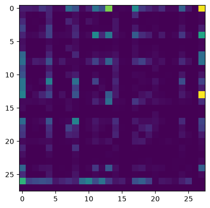
# NumPy:      N[row, column] -> N[i, j]
# Matplotlib: (x, y)         -> (column, row) -> (j, i)
# why .item()
# when we index into these arrays, we get a tensor back, eg.
print(N[3,3])
print(type(N[3,3]))
print(N[3,3].item())
print(type(N[3,3].item()))tensor(149, dtype=torch.int32)
<class 'torch.Tensor'>
149
<class 'int'>
import matplotlib.pyplot as plt
# Display plots directly inside the Jupyter notebook
%matplotlib inline

# Create a large figure so the text inside each cell is easy to read
plt.figure(figsize=(24,24))

# Display the matrix N as a heatmap
# Larger values are shown with darker shades of blue
plt.imshow(N, cmap='Blues')

# Go through every row and column of the matrix
# i = row index, j = column index (NumPy matrix indexing: N[row, column])
for i in range(28):
    for j in range(28):

        # Combine the two characters represented by this cell
        # Example: 'a' + 'b' -> "ab"
        chstr = itos[i] + itos[j]

        # IMPORTANT:
        # NumPy indexes matrices as N[row, column] -> N[i, j]
        # Matplotlib places text using (x, y) coordinates.
        #
        # x = column = j
        # y = row    = i
        #
        # So we pass (j, i), NOT (i, j).

        # Write the character pair near the top of the cell
        plt.text(
            j, i,
            chstr,
            ha="center",      # horizontally center the text
            va="bottom",      # place it toward the bottom of the given point (top half of cell)
            color="gray"
        )

        # Write the actual count/value stored in N[i, j]
        plt.text(
            j, i,
            N[i, j].item(),   # .item() converts the PyTorch tensor into a regular Python number
            ha="center",
            va="top",         # place it toward the top of the given point (bottom half of cell)
            color="red"
        )

# Hide the x and y axes since they aren't useful here
plt.axis('off')
(np.float64(-0.5), np.float64(27.5), np.float64(27.5), np.float64(-0.5))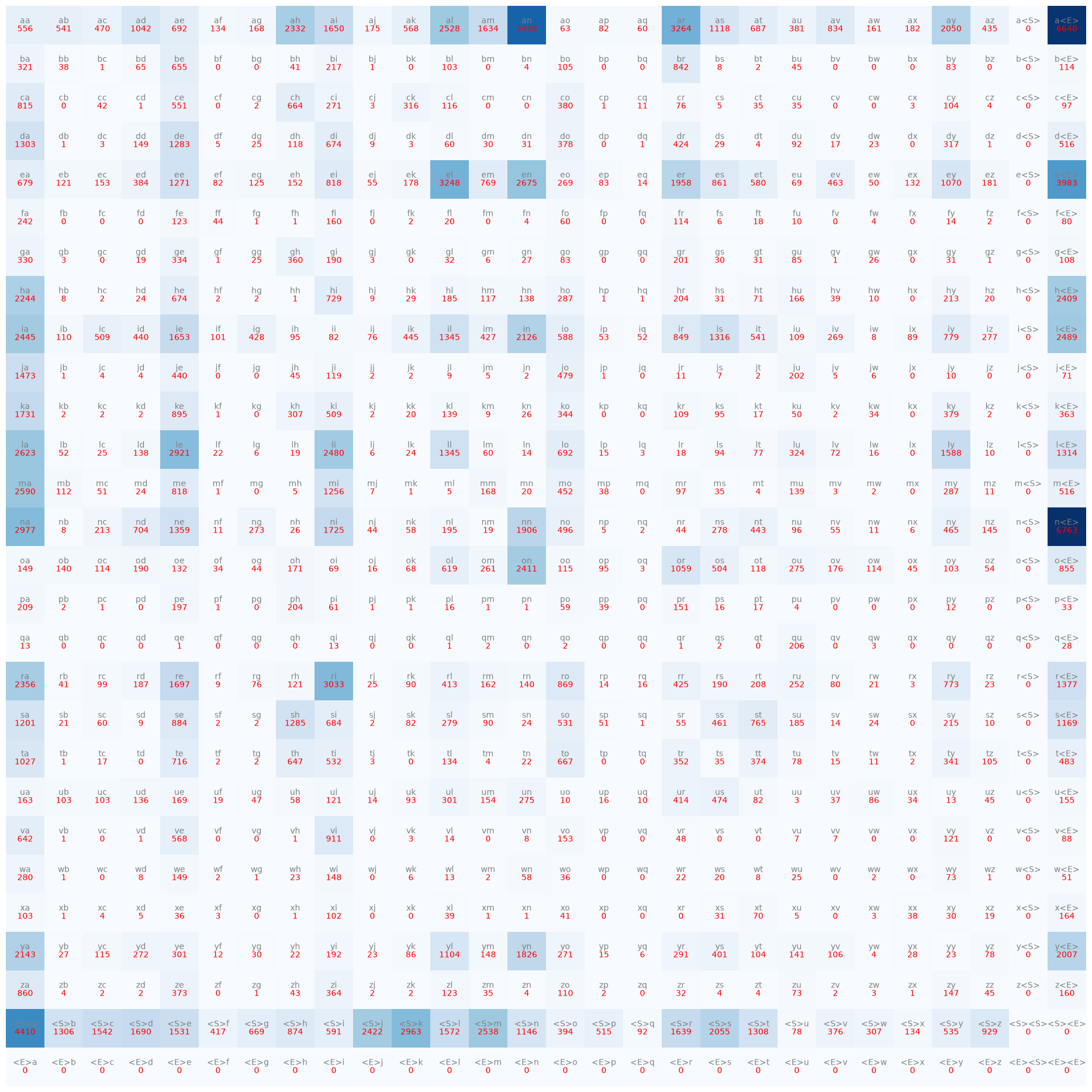
# upon careful scrutinization, we are not being very clever
# look at the last row and second last column, it is completely filled with zero's, and a 2x2 matrix at the bottom right too(only <S><E> is valid there for empty word)
# that's cuz <E> will never be the first character of a bigram, and <S> will never be the second character of a bigram
# we are using brackets <> cuz it is a convention to do so in NLP
# now, we won't use 2 special tokens. We're only going to use one special token, so N array would be 27x27 insteadN = torch.zeros((27,27), dtype = torch.int32)
chars = sorted(list(set(''.join(words))))
stoi = {s:i+1 for i, s in enumerate(chars)} # a starts at 1 when stored into stoi, expected: {'a':1, 'b':2, ..., 'z':26}
#using th special token '.' instead of <S> and <E> for efficiency
# also, we want to position it to index 0 and offset a-z by 1
stoi['.'] = 0
itos = {i:s for s, i in stoi.items()}
itos{1: 'a',
2: 'b',
3: 'c',
4: 'd',
5: 'e',
6: 'f',
7: 'g',
8: 'h',
9: 'i',
10: 'j',
11: 'k',
12: 'l',
13: 'm',
14: 'n',
15: 'o',
16: 'p',
17: 'q',
18: 'r',
19: 's',
20: 't',
21: 'u',
22: 'v',
23: 'w',
24: 'x',
25: 'y',
26: 'z',
0: '.'}for word in words:
chs = ['.'] + list(word) + ['.']
for ch1, ch2 in zip(chs, chs[1:]):
ix1 = stoi[ch1]
ix2 = stoi[ch2]
N[ix1, ix2] += 1import matplotlib.pyplot as plt
# Display plots directly inside the Jupyter notebook
%matplotlib inline
plt.figure(figsize=(24,24))
plt.imshow(N, cmap='Blues')
# Go through every row and column of the matrix
for i in range(27):
for j in range(27):
# Combine the two characters represented by this cell. # Example: 'a' + 'b' -> "ab"
chstr = itos[i] + itos[j]
plt.text(
j, i,
chstr,
ha="center",
va="bottom",
color="gray"
)
plt.text(
j, i,
N[i, j].item(),
ha="center",
va="top",
color="red"
)
plt.axis('off')(np.float64(-0.5), np.float64(26.5), np.float64(26.5), np.float64(-0.5))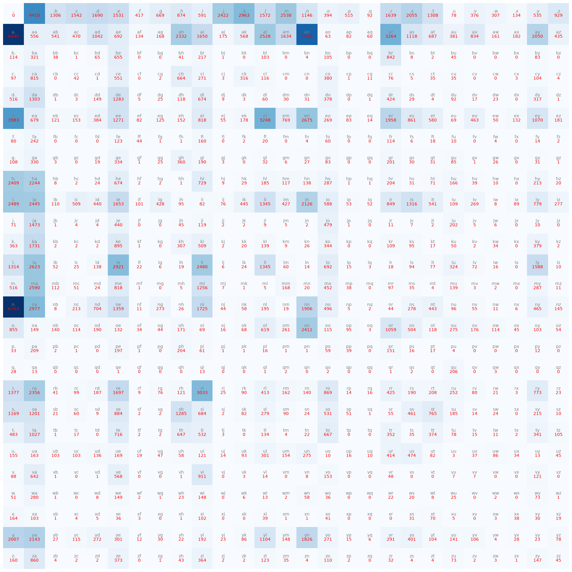
# note: first row is the start letter one, i.e. .a, .b, it is equivalent to <S>a, <S>b, etc
# note: first column is the end letter one, i.e. a., b., it is equivalent to a<E>, b<E>, etc# to sample the first character of the name, we look at the first row, .a, .b.
# don't get confused .a doesn't mean it ends at a.
# here .a means <S>a, so it means, how likely is a to be the first character of a wordN[0, :] #same as N[0] by the waytensor([ 0, 4410, 1306, 1542, 1690, 1531, 417, 669, 874, 591, 2422, 2963,
1572, 2538, 1146, 394, 515, 92, 1639, 2055, 1308, 78, 376, 307,
134, 535, 929], dtype=torch.int32)N[0, :].shape #same as N[0].shape by the waytorch.Size([27])# now, we want to sample from these counts
# since we are given raw counts, we have to convert them into probabilitiesp = N[0].float()
p /= p.sum()
p # we got a nice probability distribution, this gives the probability for each character to be the first in a wordtensor([0.0000, 0.1377, 0.0408, 0.0481, 0.0528, 0.0478, 0.0130, 0.0209, 0.0273,
0.0184, 0.0756, 0.0925, 0.0491, 0.0792, 0.0358, 0.0123, 0.0161, 0.0029,
0.0512, 0.0642, 0.0408, 0.0024, 0.0117, 0.0096, 0.0042, 0.0167, 0.0290])# we converted it into float so that we can normalize them, i.e. create a probability distribution within 0-1
p.sum()tensor(1.)# now we can try to sample from this distribution
# to sample from this distribution, we are going to use torch.multinomial
# it means: you can give me probabilities and i will give you integers which are sampled according to the probability distributionSampling from probabilities
# suppose: P = torch.tensor([0.50, 0.30, 0.15, 0.05])
# here, a is most likely the next character, d is the least likely, but any of them can still happen
# A probability distribution tells you how likely each outcome is.
# sampling means: Randomly pick one outcome, but make the randomness follow the given probabilities.
# it's not choosing the largest probability, it's not choosing uniformly
# we let the probabilities themselves determine how likely each outcome is to be picked# torch.multinomial
# P = torch.tensor([0.50, 0.30, 0.15, 0.05])
# torch.multinomial(P, num_samples=1)
# Here are the probabilities. Randomly choose one index according to them.
# it might return tensor[0] or tensor[1] or tensor[2] or even tensor[3]
# For one sample, anything can happen.
# but if we sample many times
# for _ in range(10):
# print(torch.multinomial(P, 1).item())
# we will notice that in one run, [0] appears most and [3] appears least
# and why're we doing this? cuz we want it to feel natural
# we don't want every single word to start with the same letter with the highest probability# to make everything deterministic, we are going to use a generator object in pytorch
# we provide seed value with some random num, this seed is a generator, and it gives us an object G which can be passed to a function that creates 3 random numbers
g = torch.Generator().manual_seed(2147483647)
p = torch.rand(3, generator = g) # provide 3 random numbers between 0 and 1 according to seed.
# We are deliberately using the same seed to get the same results on every iteration for learning purposes
print(p)
p /= p.sum() # get a nice probability distribution
print(p)tensor([0.7081, 0.3542, 0.1054])
tensor([0.6064, 0.3033, 0.0903])
# now we can use torch.multinomial to draw samples from this probability distribution
torch.multinomial(p, num_samples=100, replacement=True, generator=g)
# p: torch tensor of probability distributions
# we ask for number of samples, eg. 20
# replacement:True ensures that by drawing an element once, it can also be drawn in the next run. i.e. independent of previous selections
# replacement:True, need to specify cuz false by default
# generator passed to get deterministic resultstensor([1, 1, 2, 0, 0, 2, 1, 1, 0, 0, 0, 1, 1, 0, 0, 1, 1, 0, 0, 1, 0, 2, 0, 0,
1, 0, 0, 1, 0, 0, 0, 1, 1, 1, 0, 1, 1, 0, 0, 1, 1, 1, 0, 1, 1, 0, 1, 1,
0, 2, 0, 0, 0, 0, 0, 0, 0, 0, 0, 0, 1, 1, 0, 0, 0, 0, 0, 0, 0, 0, 1, 0,
0, 1, 0, 0, 0, 0, 0, 0, 0, 1, 2, 0, 0, 0, 0, 0, 0, 1, 0, 0, 2, 0, 1, 0,
0, 1, 1, 1])# prob for first sample, i.e. 0: 61%, for second sample: 30%, for third sample: 9%
# the more we sample, the more accurate it should be# getting back to topicp = N[0].float()
p /= p.sum()
ptensor([0.0000, 0.1377, 0.0408, 0.0481, 0.0528, 0.0478, 0.0130, 0.0209, 0.0273,
0.0184, 0.0756, 0.0925, 0.0491, 0.0792, 0.0358, 0.0123, 0.0161, 0.0029,
0.0512, 0.0642, 0.0408, 0.0024, 0.0117, 0.0096, 0.0042, 0.0167, 0.0290])# note: we are working on N[0], so we are working to find which character might be the first character to our wordg = torch.Generator().manual_seed(2147483647)
print(torch.multinomial(p, num_samples=1, replacement=True, generator=g)) # first call, returns sample 3, which is c
ix = torch.multinomial(p, num_samples=1, replacement=True, generator=g).item() # second call, returns new sample 5
print(ix)
print(itos[ix])tensor([3])
5
e
# we got the first character, now we have to draw the next one
# we drew e, so now look at the row e and find the character that is likely to occur after e
# now we write a loopg = torch.Generator().manual_seed(2147483647)
for i in range(30):
out = []
ix = 0
while True:
p = N[ix].float() #process the first character, get the probability distribution of the first row for ix = 0, # in the second call it uses p = N[5] and so on until . is reached
p /= p.sum() #normalize p
# draw a single sample from this distribution
# this will tell us the index of the character that is going to be next
ix = torch.multinomial(p, num_samples=1, replacement=True, generator=g).item()
out.append(itos[ix])
if ix == 0: #we reached the end token
break
print(''.join(out))cexze.
momasurailezitynn.
konimittain.
llayn.
ka.
da.
staiyaubrtthrigotai.
moliellavo.
ke.
teda.
ka.
emimmsade.
enkaviyny.
ftlspihinivenvorhlasu.
dsor.
br.
jol.
pen.
aisan.
ja.
feniee.
zem.
deru.
firit.
gaikajahahbevare.
kiysthelenaririenah.
keen.
x.
al.
kal.
# the reason these samples are so terrible is that bigram language model is just terrible
# but they are name like a little bit but not name like enough
# but think from the model's perspective, eg. you see x., the model doesn't know that x is the first x of the word. it is just thinking about one character at a time
# so it directly also looks for how likely is x the last character
# to convince yourself that this is not so terrible is by : instead of relying on p(that came from our dataset of 32k words),
# if p was just a uniform probability distribution of all 27 characters making any character to appear equally likelyg = torch.Generator().manual_seed(2147483647)
for i in range(15):
out = []
ix = 0
while True:
# p = N[ix].float()
# p /= p.sum()
p = torch.ones(27) / 27.0
ix = torch.multinomial(p, num_samples=1, replacement=True, generator=g).item()
out.append(itos[ix])
if ix == 0: #we reached the end token
break
print(''.join(out))cexzm.
zoglkurkicqzktyhwmvmzimjttainrlkfukzkktda.
sfcxvpubjtbhrmgotzx.
iczixqctvujkwptedogkkjemkmmsidguenkbvgynywftbspmhwcivgbvtahlvsu.
dsdxxblnwglhpyiw.
igwnjwrpfdwipkwzkm.
desu.
firmt.
gbiksjbquabsvoth.
kuysxqevhcmrbxmcwyhrrjenvxmvpfkmwmghfvjzxobomysox.
gbptjapxweegpfwhccfyzfvksiiqmvwbhmiwqmdgzqsamjhgamcxwmmk.
iswcxfmbalcslhy.
fpycvasvz.
bqzazeunschck.
wnkojuoxyvtvfiwksddugnkul.
# saw the output from a completely untrained model? saw how random it could have actually been?Normalization and broadcasting
# now, let's fix an efficiency issue
# we are always fetching a row of N from the count matrix up, then converting to float, and then dividing
# this happens in every iteration of the loop
# and we're renormalizing these rows again and again
# so let's prepare a new matrix P based on existing matrix N, but P will have probabilities
# i.e. same as N, but instead of values, we set probabilities (value/sum of that row) normalized to one
# so it indicates the probability distribution directly for the next character(column) given the character before(row)# we're doing this not just for efficiency, but also to practice n-dimensional tensors and practice their manipulation
# practice broadcasting
# if we're going to build up to transformers, we have to be good in tensor manipulations, complicated array operations for efficiency# N
P = N.float()
# P #same as N but all values are floating point ones
# and now, we want to divide all the rows so that they sum to 1, but P = P / P.sum() doesn't work cuz it sums all the values of entire matrix, not just for each row# P.sum()
# We want to divide all the rows value's by the respective sum of the row
# looking documentation for torch.sum
# so, we provide the array we want to sum, and it's dimensions
# but not just that, be careful of keep dimension attribute
# if keepdim = True, output tensor is of the same size as input, except in the dimension along you summed which will become 1
# but if keepdim = False, this dimension is squeezed out, so torch.sum does the sum and also collapses dimension to be of size one,
# but addition it also does the squeeze, it squeezes out that dimensionP.shapetorch.Size([27, 27])print(P.sum)
# take the 0th dimension
print(P.sum(0, keepdim=True))
print(P.sum(0, keepdim=True).shape)
print(P.sum(0, keepdim=False))
print(P.sum(0, keepdim=False).shape)
# in this case we did the sum vertically, i.e. for each columns, and we received a single 1x27 vector of sum values
# the difference of keepdim would be that we either get a 1d vector or a 2d vector output<built-in method sum of Tensor object at 0x73944a735050>
tensor([[32033., 33885., 2645., 3532., 5496., 20423., 905., 1927., 7616.,
17701., 2900., 5040., 13958., 6642., 18327., 7934., 1026., 272.,
12700., 8106., 5570., 3135., 2573., 929., 697., 9776., 2398.]])
torch.Size([1, 27])
tensor([32033., 33885., 2645., 3532., 5496., 20423., 905., 1927., 7616.,
17701., 2900., 5040., 13958., 6642., 18327., 7934., 1026., 272.,
12700., 8106., 5570., 3135., 2573., 929., 697., 9776., 2398.])
torch.Size([27])
# we don't want 1x27 row vector, we don't want the sum of counts across a column
# we want to sum of counts across a row, so we want a 27x1 row vector, and each entry gives corresponding sum of that row# to sum the other way,
# take the 0th dimension
print(P.sum(1, keepdim=True))
print(P.sum(1, keepdim=True).shape)
print(P.sum(1, keepdim=False))
print(P.sum(1, keepdim=False).shape)tensor([[32033.],
[33885.],
[ 2645.],
[ 3532.],
[ 5496.],
[20423.],
[ 905.],
[ 1927.],
[ 7616.],
[17701.],
[ 2900.],
[ 5040.],
[13958.],
[ 6642.],
[18327.],
[ 7934.],
[ 1026.],
[ 272.],
[12700.],
[ 8106.],
[ 5570.],
[ 3135.],
[ 2573.],
[ 929.],
[ 697.],
[ 9776.],
[ 2398.]])
torch.Size([27, 1])
tensor([32033., 33885., 2645., 3532., 5496., 20423., 905., 1927., 7616.,
17701., 2900., 5040., 13958., 6642., 18327., 7934., 1026., 272.,
12700., 8106., 5570., 3135., 2573., 929., 697., 9776., 2398.])
torch.Size([27])
# note that shape is 27 x 1, so it's a column vector, we're going horizontally
# buut, notice that these counts are identical no matter whether we sum across rows or columns
# that's cuz this array of counts comes from bigram statistics and by coincidence or by the way this array is constructed, the sums along rows and columns are identical# N
P = N.float()
# P #same as N but all values are floating point ones
# and now, we want to divide all the rows so that they sum to 1, but P = P / P.sum() doesn't work cuz it sums all the values of entire matrix, not just for each row
P = P / P.sum(1, keepdim=True) #is this broadcastable/allowed?# is it possible to take a 27x27 array and divide by 27 x 1 array?
# P / P.sum(1, keepdim=True)
# 27 x 27
# -------
# 27 x 1
# whether or not we can perform this operation is determined by broadcasting rules (explore this in pytorch)
# from documentation, there are a few conditions:
# 1. each tensor has atleast 1 dimension
# 2. when iterating over the dimension sizes, starting at the trailing(later) dimension, the dimension sizes must either be equal, one of them is 1, or one of them doesn't exist.# so we align them like this
# 27 x 27
# -------
# 27 x 1
# move from right to left
# from the right, they are not equal, but one of them is a 1, so it is fine, and in the other dimension, both are equal (27)
# since they are fine, the operation P = P / P.sum(1, keepdim=True) is broadcastable/allowed
# so what happens internally is that, the dimension 1 is stretched out, it is copied to match 27
# so our column vector(that has the sum) is copied 27 times for each one of those 27 columns(. - z), and internally it becomes 27/27
# finally element wise division is done
# thus this action shall normalize every single row# check it's truth by taking the first row's sum which should be 1 cuz it's normalized
P[0].sum()tensor(1.)# and since it works, we expect the exact same results for this too:
g = torch.Generator().manual_seed(2147483647)
for i in range(15):
out = []
ix = 0
while True:
# p = N[ix].float()
# p /= p.sum()
p = P[ix]
ix = torch.multinomial(p, num_samples=1, replacement=True, generator=g).item()
out.append(itos[ix])
if ix == 0: #we reached the end token
break
print(''.join(out))cexze.
momasurailezitynn.
konimittain.
llayn.
ka.
da.
staiyaubrtthrigotai.
moliellavo.
ke.
teda.
ka.
emimmsade.
enkaviyny.
ftlspihinivenvorhlasu.
dsor.
# now, let's understand where broadcasting could go wrong
# also lookup some tutorials on broadcasting and practice it, cuz you can run into bugs very quicklyP = N.float()P.sum(1, keepdim=True).shapetorch.Size([27, 1])P.sum(1, keepdim=True)tensor([[32033.],
[33885.],
[ 2645.],
[ 3532.],
[ 5496.],
[20423.],
[ 905.],
[ 1927.],
[ 7616.],
[17701.],
[ 2900.],
[ 5040.],
[13958.],
[ 6642.],
[18327.],
[ 7934.],
[ 1026.],
[ 272.],
[12700.],
[ 8106.],
[ 5570.],
[ 3135.],
[ 2573.],
[ 929.],
[ 697.],
[ 9776.],
[ 2398.]])# now suppose we erase keepdim=True, and by default it's false
# what happens then? well it just squeezes the dimension 1 out turning it into 1 d arrayP.sum(1)tensor([32033., 33885., 2645., 3532., 5496., 20423., 905., 1927., 7616.,
17701., 2900., 5040., 13958., 6642., 18327., 7934., 1026., 272.,
12700., 8106., 5570., 3135., 2573., 929., 697., 9776., 2398.])P.sum(1).shapetorch.Size([27])# you might think that P / P.sum(1) might work as expected, but it doesn't
# let's check if it is broadcastable# P / P.sum(1)
# 27 x 27
# -------
# 27
# rule 1: align all dimensions on the right
# move from right to left
# either equal, one of them should be 1, or one of them shouldn't exist
# equal, and doesn't exist
# so internally, broadcasting will create a 1 in front, and it will get copied and will broadcast
# 27 x 27
# -------
# 1 x 27
# this won't work and you'll get garbage resultP = N.float()
P = P / P.sum(1)#just removing keepdim=True stopped it from working# and since it works, we expect the exact same results for this too:
g = torch.Generator().manual_seed(2147483647)
for i in range(15):
out = []
ix = 0
while True:
# p = N[ix].float()
# p /= p.sum()
p = P[ix]
ix = torch.multinomial(p, num_samples=1, replacement=True, generator=g).item()
out.append(itos[ix])
if ix == 0: #we reached the end token
break
print(''.join(out))cexze.
zoghkurkicqukwydwevizimittain.
juffk.
kavig.
jomiviubrtthrugotzi.
mozixxluxuggwytedowekoumimmstheuwnkaviynyzytlsphiguwdebdorhlusuzusprddinwil.
pynwuigwn.
wuwffwippppem.
deru.
fixxt.
gbikajahudoshath.
kucoxxevicyabruqubh.
keengwmalosilmudavazeobomysoxxxsptjappheviphisphiyzzelyillevebhmiffidezhakamckamcoworucishaxfubalckahy.
foronazzz.
bezazexxzahay.
# so why was the keepdim necessary?
# earlier when keepdim was used, the 1-d vector(column) was copied across each column properly,
# so eg. for a value in fourth row and first column, row[3][0], it was divided by sum of the fourth row[3]
# but now, when keepdim is absent, the 1-d vector(column) was copied across each row instead
# so eg. for a value in fourth row and first column, row[3][0], it was divided by sum of the first row[0]
# so first column was divided by sum of first row, instead of first row being divided by sum of first row and so on
# so first row was divided as: first entry divided by sum of first row ok, but second entry of first row divided by sum of second row, 3rd entry of first row divided by sum of third row and so on.P[0].sum() # the sum of first row is not 1tensor(7.0225)P[:,0].sum() # the sum of first column is 1 instead
# now why did the first column's sum equal 1? remember that earlier coincidence that sum of rows and columns were equal, that's why bro that's why
# nice job figuring this out yourself, gud jobtensor(1.)# in short, from broadcasting rules, a dimension is silently added to the left which caused this issue, so work with it carefully
# what was supposed to be a column vector becomes a row vector instead and it works in opposite manner instead# one more note on efficiency
# we want to avoid doing this as it creates a completely new tensor
# instead, we prefer to use inplace operations if possible
# it is potentially faster, doesn't create new memory under the hood
# P = P / P.sum(1, keepdim=True)
P /= P.sum(1, keepdim=True)Likelihood and model quality
# we trained a bigram language model just by counting how frequently any pairing occurs and then normalizing so that we can get a nice probability distribution
# the elements of array P are the parameters of our bigram language model giving and summarizing the statistics of these bigrams
# so we trained the model and now we know how to sample from the model
# we just iteratively sample the next character and feed it in each time and get the next character# now, we want to evaluate the quality of this model
# we want to somehow summarize the model's quality into a single number
# how good is it at predicting the training set, eg. we can evaluate the training loss from the training set
# this training loss tells us the quality of the model in a single number1/27.00.037037037037037035# side note: if we were to sum all probability values in the matrix P, would we get 27? cuz sum for one row would be 1, and we have 27 rows# now, we want to look at the probability assigned by the model to every single bigram
# just to have a measuring reference in mind, with 27 possible characters/tokens, if everything was equally likely, we'd expect all these probabilities to be roughly 1/27.0
# roughly above 4% means that the model has learnt something useful from the given bigram statistics
# if we have a very good model, these probabilities should be near 1, which means our model is predicting what's going to come next, specially on the training set where our model was trained
# how to summarize these probabilities into a single number that measures the quality of this model?
# MAXIMUM likelihood estimation
# so what's used is called: a likelihood (likelihood is the product of all these probabilities)
# and, the product of these probabilities should be as high as possible when we are training the model and when we have a good model
# now since all our probabilities are between 0-1, our product will actually be a very small number
# so for convenience, people don't work with likelihood, instead they work with log likelihood
# to get the log likelihood, we just have to take the log of the probability
log_likelihood = 0.0
n = 0
for word in words[:3]:
chs = ['.'] + list(word) + ['.']
for ch1, ch2 in zip(chs, chs[1:]):
ix1 = stoi[ch1]
ix2 = stoi[ch2]
prob = P[ix1, ix2] #remember this recent P matrix we created from N
logprob = torch.log(prob)
log_likelihood += logprob
n += 1
print(f'{ch1}{ch2}: {prob:.4f} {logprob:.4f}')
print(f'{log_likelihood=}')
nll = -log_likelihood
print(f'{nll=}')
print(f'{nll/n=}') #average negative log likelihood: our loss function
# this negative log likelihood is a very nice loss function because the lowest it can get is 0, and the higher it is, the worse off the predictions are.e: 0.0107 -4.5399
em: 0.0504 -2.9876
mm: 0.0522 -2.9517
ma: 0.1579 -1.8459
a.: 0.0470 -3.0585
.o: 0.0071 -4.9517
ol: 0.0389 -3.2464
li: 0.1333 -2.0153
iv: 0.0444 -3.1136
vi: 0.3572 -1.0295
ia: 0.0307 -3.4845
a.: 0.0470 -3.0585
.a: 0.0185 -3.9882
av: 0.0734 -2.6114
va: 0.1315 -2.0288
a.: 0.0470 -3.0585
log_likelihood=tensor(-47.9700)
nll=tensor(47.9700)
nll/n=tensor(2.9981)
graph for log(x): focus on x = 0 to 1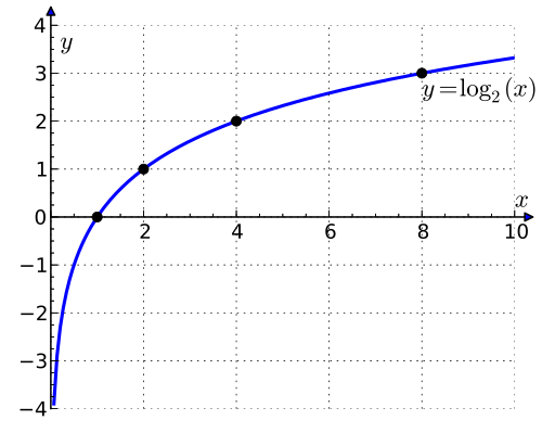
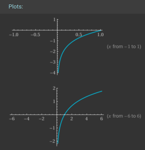
# from this graph, we can see the log is a monotonic transformation of probability
# if we pass in probability as x = 1, we get 0
# and as we go lower, i.e. probability or x < 1, we get the log's value as more and more negative until -infinity is reached at x = 0# the only reason we are doing this stuff with log is for convenience
# keep in mind: we are trying to compute product of all the probabilities, i.e. ..*.a*...*aa*ab*ac...*zz
# note: log(a*b*c) = log(a) + log(b) + log(c)
# since likelihood = product of probabilities,
# log likelihood = log(product of probabilities) = sum of logs of individual probabilities
# so log likelihood starts at 0, and it accumulates overtime by logs of all individual probabilities# so how high can log likelihood get? it can go to zero
# this happens when all probabilities are 1, and since log(1) = 0, log(1) + log(1) + ...(for all probabilities) = 0
# but when all the probabilities are very low instead of 1, our log probability gets very very negative, and we don't like this
# but why don't we like this? cuz we'd like to implement a loss function: and loss function has the semantics that low is good (which is opposite of our case) because we're always trying to minimize the loss
# so we'd like to invert this from current situation where 0(desired) and -infinity(undesired)
# to invert it, we do the negative log likelihood: which is simply the negative of log likelihood# and one final modification people like to do for convenience is instead of just the sum of nll, people compute the average of nll# so the loss function assigned by our model: the average negative log likelihood is: 2.9981: the quality of our model
# lower the anll better our model and vice versa
# and now, the job of our training is to find the parameters that minimize the negative log likelihood# SUMMARY:
# GOAL: MAXIMIZE LIKELIHOOD(product of all probabilities) OF DATA W.R.T MODEL PARAMETERS (statistical modeling) (defined in the matrix)
# equivalent to maximizing the log likelihood (because log is monotonic)
# equivalent to minimizing the negative log likelihood
# equivalent to minimizing the average negative log likelihood (guess we can't say normalized since it isn't in range 0-1.)# currently we are storing all probabilities in a table format, but what's coming up later is that these numbers won't be kept explicitly but be calculated by a neural network# now let's estimate our loss: i.e. average negative log likelihood for the entire training set
log_likelihood = 0.0
n = 0
for word in words:
chs = ['.'] + list(word) + ['.']
for ch1, ch2 in zip(chs, chs[1:]):
ix1 = stoi[ch1]
ix2 = stoi[ch2]
prob = P[ix1, ix2] #remember this recent P matrix we created from N
logprob = torch.log(prob)
log_likelihood += logprob
n += 1
# print(f'{ch1}{ch2}: {prob:.4f} {logprob:.4f}')
print(f'{log_likelihood=}')
nll = -log_likelihood
print(f'{nll=}')
print(f'{nll/n=}') #average negative log likelihood: our loss functionlog_likelihood=tensor(-650247.6250)
nll=tensor(650247.6250)
nll/n=tensor(2.8501)
# we can also evaluate the probability for any word that we want
log_likelihood = 0.0
n = 0
# the loss is lower than avg so it is slightly likely name (atleast based on the training data)
# for word in ["satish"]:
# searched the table for hx=0 lol
for word in ["satishx"]:
chs = ['.'] + list(word) + ['.']
for ch1, ch2 in zip(chs, chs[1:]):
ix1 = stoi[ch1]
ix2 = stoi[ch2]
prob = P[ix1, ix2] #remember this recent P matrix we created from N
logprob = torch.log(prob)
log_likelihood += logprob
n += 1
# print(f'{ch1}{ch2}: {prob:.4f} {logprob:.4f}')
print(f'{log_likelihood=}')
nll = -log_likelihood
print(f'{nll=}')
print(f'{nll/n=}') #average negative log likelihood: our loss functionlog_likelihood=tensor(-inf)
nll=tensor(inf)
nll/n=tensor(inf)
Smoothing
# acc to our model, hx has a 0% probability, so log(0) = -inf, and our anll = inf
# this is unreasonable, cuz we plugged a string that would be somewhat reasonable but it shouldn't be 0% likely
# there's a very simple fix to smooth out our model: model smoothing
# we will add fake counts: eg. add a count of 1 to everything
# the more we add, the more smoother it gets, and we get a more smoother uniform model
# 1 is a decent count to add which will ensure that there will be no 0s in our probability matrix P, this can change our generations by a little bit
# so it is unlikely to get an infinityP = (N+1).float()
P /= P.sum(1, keepdims=True)# we can also evaluate the probability for any word that we want
log_likelihood = 0.0
n = 0
# the loss is lower than avg so it is slightly likely name (atleast based on the training data)
# for word in ["satish"]:
# searched the table for hx=0 lol
for word in ["satishx"]:
chs = ['.'] + list(word) + ['.']
for ch1, ch2 in zip(chs, chs[1:]):
ix1 = stoi[ch1]
ix2 = stoi[ch2]
prob = P[ix1, ix2] #remember this recent P matrix we created from N
logprob = torch.log(prob)
log_likelihood += logprob
n += 1
print(f'{ch1}{ch2}: {prob:.4f} {logprob:.4f}')
print(f'{log_likelihood=}')
nll = -log_likelihood
print(f'{nll=}')
print(f'{nll/n=}') #average negative log likelihood: our loss function.s: 0.0641 -2.7468
sa: 0.1478 -1.9119
at: 0.0203 -3.8977
ti: 0.0952 -2.3515
is: 0.0743 -2.5998
sh: 0.1581 -1.8444
hx: 0.0001 -8.9415
x.: 0.2279 -1.4788
log_likelihood=tensor(-25.7726)
nll=tensor(25.7726)
nll/n=tensor(3.2216)
# so until now, we've trained a respectable bigram character level language model
# and we've trained the model by looking at the counts of all the bigrams and normalizing the rows to get probability distributions
# we can also use the parameters(probability values inside matrix P) of this model to perform sampling of new words according to the probability distribution
# and we can evaluate the quality of this model: summarized in a single number: negative log likelihood, and the lower this loss, the better our model is
# because it is giving high probabilities to the actual next characters in all bigrams in our training set
# but what we did was just counts and normalizing these counts
# but now we want to take an alternative approach and end up in a very similar position
# the approach is very different cuz we would like to cast the problem of bigram character level language modeling into the neural network framework
# and in the neural network framework, we're going to approach things differently but end up in a similar spotThe neural network approach
PART 2: THE NEURAL NETWORK APPROACH# our neural network is still going to be a bigram character level language model
# so it receives a single character as input
# and there's a neural network with some parameters
# and it will output the probability distribution over the next character in a sequence,
# it will make guesses as to what is likely to follow the char that was input to this model
# ADDITIONALLY, we will be able to evaluate any setting of the parameters of the neural net cuz we have the loss function: the negative log likelihood
# so we'll look at the probability distributions and then look at the labels (identity of next character in that bigram)
# knowing the second character in the bigram allows us to look at how high of a probaility the model assigns to that character
# ofcourse, we want the probability to be very high, ie. loss is low
# then we're going to use gradient-based optimization to tune the parameters of this network cuz we have the loss function and we'll minimize it
# so we'll tune the weights so that neural net correctly predicts the probabilities for the next characteropen("names.txt", "r").read()#read everything into a massive string
# since it's a massive string, we only want the individual words, and put them in a list
words = open("names.txt", "r").read().splitlines()
words[:20]#look at first 20 words['emma',
'olivia',
'ava',
'isabella',
'sophia',
'charlotte',
'mia',
'amelia',
'harper',
'evelyn',
'abigail',
'emily',
'elizabeth',
'mila',
'ella',
'avery',
'sofia',
'camila',
'aria',
'scarlett']import torchimport matplotlib.pyplot as plt
%matplotlib inlineN = torch.zeros((27,27), dtype = torch.int32)
chars = sorted(list(set(''.join(words))))
stoi = {s:i+1 for i, s in enumerate(chars)} # a starts at 1 when stored into stoi, expected: {'a':1, 'b':2, ..., 'z':26}
#using th special token '.' instead of <S> and <E> for efficiency
# also, we want to position it to index 0 and offset a-z by 1
stoi['.'] = 0
itos = {i:s for s, i in stoi.items()}
itos{1: 'a',
2: 'b',
3: 'c',
4: 'd',
5: 'e',
6: 'f',
7: 'g',
8: 'h',
9: 'i',
10: 'j',
11: 'k',
12: 'l',
13: 'm',
14: 'n',
15: 'o',
16: 'p',
17: 'q',
18: 'r',
19: 's',
20: 't',
21: 'u',
22: 'v',
23: 'w',
24: 'x',
25: 'y',
26: 'z',
0: '.'}# 1. We want to create the training set of this neural network, i.e. of all the bigrams, bigrams denote (x, y)
# our training set will have two lists: a. the inputs b. the targets. We're given the first character of the bigram, and we're trying to find the next one
xs, ys = [], []
for w in words[:1]:
chs = ['.'] + list(w) + ['.']
for ch1, ch2 in zip(chs, chs[1:]):
ix1 = stoi[ch1]
ix2 = stoi[ch2]
print(ch1, ch2)
xs.append(ix1)
ys.append(ix2)
# we don't want list of ints, we will create tensors from these
xs = torch.tensor(xs)
ys = torch.tensor(ys). e
e m
m m
m a
a .
xstensor([ 0, 5, 13, 13, 1])ystensor([ 5, 13, 13, 1, 0])# so, when input is 0, we want the weights to be arranged so that 5 gets a high probability, similar for 5-13, 13-13, 13-1, and 1-0# caution: be careful of APIs of some frameworks, eg. we used torch.tensor, but there is also a torch.Tensor which is very very similar too
# the official documentation doesn't distinguish much, but in stackoverflow there was a thread that distinguishes the difference# difference:
# torch.tensor: infers the dtype automatically, also has argument dtype if we want to change it, so stick with this instead(recommended)
# torch.Tensor: returns torch.FloatTensorprint(xs.dtype)
print(ys.dtype)torch.int64
torch.int64
# now, how will we feed these examples xs, ys into neural network?
# right now, it's not straightforward, cuz these examples are integers that are index of characters(., a, ..., z), and we can't just plug integer index into neural network
# neural networks has neurons, neurons have weights and they act multiplicatively on the input: wx + b, tanh, so it doesn't make sense to use these 0-26 int directly
# instead, a common way of encoding integers: one-hot encoding:
# we take an integer eg.13 and create a vector with all zeros except for the 13th dimension(which will be 1), and we feed it into a neural net# pytorch has a one hot function inside torch.nn.functional that takes a tensor made up of integers
# and it also takes input as num of classes: how long you want your vector to be. in our case 27 = 26(a-z) + 1(.)
# not specifying num_classes might give incorrect result: might take largest value in xs, eg. 13 insteadimport torch.nn.functional as F
xenc = F.one_hot(xs, num_classes=27)
xenctensor([[1, 0, 0, 0, 0, 0, 0, 0, 0, 0, 0, 0, 0, 0, 0, 0, 0, 0, 0, 0, 0, 0, 0, 0,
0, 0, 0],
[0, 0, 0, 0, 0, 1, 0, 0, 0, 0, 0, 0, 0, 0, 0, 0, 0, 0, 0, 0, 0, 0, 0, 0,
0, 0, 0],
[0, 0, 0, 0, 0, 0, 0, 0, 0, 0, 0, 0, 0, 1, 0, 0, 0, 0, 0, 0, 0, 0, 0, 0,
0, 0, 0],
[0, 0, 0, 0, 0, 0, 0, 0, 0, 0, 0, 0, 0, 1, 0, 0, 0, 0, 0, 0, 0, 0, 0, 0,
0, 0, 0],
[0, 1, 0, 0, 0, 0, 0, 0, 0, 0, 0, 0, 0, 0, 0, 0, 0, 0, 0, 0, 0, 0, 0, 0,
0, 0, 0]])xenc.shapetorch.Size([5, 27])plt.imshow(xenc)<matplotlib.image.AxesImage at 0x7db4875d3230>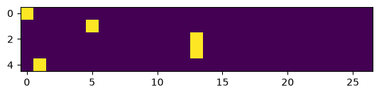
# understanding this graph: try to read ., e, m, m, a# when we're plugging numbers into neural nets, we want them to be floating points instead of integers
xenc.dtypetorch.int64# one_hot received 64 bit integer and returned the same datatype
# in the signature of one_hot, it doesn't even take the desired datatype of the output tensor, so we gonna cast it like this
xenc = F.one_hot(xs, num_classes=27).float()
xenctensor([[1., 0., 0., 0., 0., 0., 0., 0., 0., 0., 0., 0., 0., 0., 0., 0., 0., 0.,
0., 0., 0., 0., 0., 0., 0., 0., 0.],
[0., 0., 0., 0., 0., 1., 0., 0., 0., 0., 0., 0., 0., 0., 0., 0., 0., 0.,
0., 0., 0., 0., 0., 0., 0., 0., 0.],
[0., 0., 0., 0., 0., 0., 0., 0., 0., 0., 0., 0., 0., 1., 0., 0., 0., 0.,
0., 0., 0., 0., 0., 0., 0., 0., 0.],
[0., 0., 0., 0., 0., 0., 0., 0., 0., 0., 0., 0., 0., 1., 0., 0., 0., 0.,
0., 0., 0., 0., 0., 0., 0., 0., 0.],
[0., 1., 0., 0., 0., 0., 0., 0., 0., 0., 0., 0., 0., 0., 0., 0., 0., 0.,
0., 0., 0., 0., 0., 0., 0., 0., 0.]])xenc.dtypetorch.float32plt.imshow(xenc)<matplotlib.image.AxesImage at 0x7db487412990>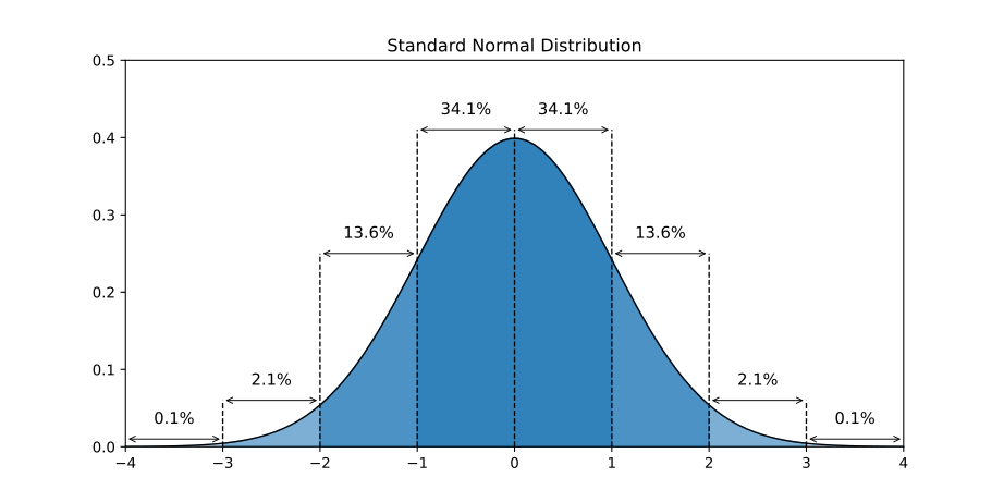
# Let's construct our first neuron, they'll take our inputs, and perform wx+b. wx is the dot product
# let's define the initial weights for the neuron, set them to be random values
# randn(): returns tensor filled with random nums from a normal distribution(bell shaped curve). some values might be above 3 in magnitude.
# W: a column vector of 27 numbers
W = torch.randn((27, 1)) # 27x1 matrix. 27 weights for 1 neuron
Wtensor([[-0.3689],
[ 0.3017],
[ 0.7983],
[-0.2436],
[-0.7199],
[-0.7178],
[-0.5994],
[ 0.4572],
[ 0.5109],
[ 0.1610],
[ 0.4179],
[ 0.9262],
[-0.1166],
[-1.6169],
[-1.2806],
[ 0.6441],
[ 0.6572],
[ 0.0416],
[ 0.2845],
[ 0.2733],
[ 0.4007],
[ 0.7402],
[ 0.2278],
[-0.6630],
[-0.4101],
[-0.6030],
[ 1.0632]])# now multiply these weights by our input: wx
# @: matrix multiplication operator in pytorch
# xenc.shape: 5x27, W.shape: 27.1, result.shape: 5x1
xenc @ Wtensor([[-0.3689],
[-0.7178],
[-1.6169],
[-1.6169],
[ 0.3017]])# we evaluate 5 activations of this neuron on these 5 inputs all in parallel
# we fed 5 inputs into the same neuron simultaneously, and in parallel, pytorch has evaluated wx for all of them
# now instead of a single neuron, we want to have 27 neuronsW = torch.randn((27, 27)) #27 weights for 27 neurons each
xenc @ W
# this will evaluate all 27 neurons on all 5 inputs giving us a better and bigger resulttensor([[-0.2381, 0.3721, -0.6063, 0.2695, -0.4948, -0.2142, 0.3754, -0.9684,
-0.2667, -0.6459, 0.9267, 1.3762, -0.4314, 0.4009, -0.6887, -0.6417,
1.3215, -0.0305, 1.0770, 0.9236, 0.7579, -0.2886, -0.5679, 0.2053,
-0.9550, -0.1571, 0.0972],
[ 1.2477, -0.6483, 2.9427, -1.1470, -0.5661, 0.2784, -0.9179, 1.8721,
-1.0616, -0.4578, 1.5357, 0.1272, 0.1167, -0.0767, 0.7872, 0.3312,
-0.0364, 0.4641, -0.3681, 0.0905, 0.4137, -0.6679, 0.1785, -0.6744,
-0.1722, 0.8944, 0.7667],
[-0.2772, -0.9649, -1.8149, 0.9409, 0.9290, -0.9330, 0.4190, 0.2508,
0.9838, 1.1341, -0.0316, -0.9327, 0.3265, -1.1368, -0.9668, 1.5915,
0.7876, 0.2264, 0.8547, -2.7509, 2.0192, -1.1206, -1.7251, -0.1866,
0.1177, -0.7251, 0.4731],
[-0.2772, -0.9649, -1.8149, 0.9409, 0.9290, -0.9330, 0.4190, 0.2508,
0.9838, 1.1341, -0.0316, -0.9327, 0.3265, -1.1368, -0.9668, 1.5915,
0.7876, 0.2264, 0.8547, -2.7509, 2.0192, -1.1206, -1.7251, -0.1866,
0.1177, -0.7251, 0.4731],
[-0.2046, -0.1169, -0.5736, -0.6125, -1.1879, 1.5528, 0.3456, -0.9457,
-0.1947, 0.7187, -1.1427, 0.6083, 0.6176, 1.4568, -0.4730, -1.2182,
0.6352, 0.4920, 1.1291, -2.0718, -0.0313, 1.7058, -1.3478, 0.2128,
-1.1291, -1.1662, -1.7359]])# 5x27 , 27x27 => 5x27
(xenc @ W).shapetorch.Size([5, 27])# what does every element there tell us?
# it tells us that, for every single one of those 27 neurons we created, what is the firing rate of those neurons on every one of those 5 examples
(xenc @ W)[2, 12] # this gives us a firing rate of the 13th neuron looking at the third inputtensor(0.3265)(xenc @ W)[2,0]tensor(-0.2772)# so by using matrix multiplication, we can very efficiently evaluate the dot product between lots of input examples in a batchxenc[2]tensor([0., 0., 0., 0., 0., 0., 0., 0., 0., 0., 0., 0., 0., 1., 0., 0., 0., 0.,
0., 0., 0., 0., 0., 0., 0., 0., 0.])W[12]tensor([-0.5477, -1.1185, -0.6815, 0.2531, 0.3081, -1.1757, 0.2530, 0.7343,
0.3226, 0.9534, 0.0457, 0.8043, -0.5917, -0.8857, 0.0232, -0.3316,
-0.3378, 1.1293, 0.8111, -1.2503, -0.5216, -0.4478, -1.6201, -1.3961,
-1.1951, -0.0884, 1.7745])(xenc[2] * W[:, 12]).sum()
# to show the same element wise multiplication
# but this is done efficiently by matrix multiplication operation for all input examples and for all output neurons of this first layertensor(0.3265)# so what we did until now was, we fed our 27-dimensional inputs into a first layer of a neural net that has 27 neurons
# i.e. 27 inputs and 27 neurons, these neurons perform wx, they don't have a bias and they don't have a non-linearity like tanh
# we'll leave this layer to be linear
# additionally, we're not going to have any other layers. This is going to be it, the dumbest, smallest, simplest neural net: just a single linear layer# now we want to explain what we want those 27 outputs to be
# for every input example, we're trying to produce a probability distribution for the next character in the sequence
# we see that some nums are -ve, some are +ve as they are coming out of torch.randn() : normal distribution parameters
# but what we want is something like in previous matrix, where each row told us the counts which we normalized to get probability distributions
# we want something similar to come out of a neural net: but what we have now is some +ve and -ve nums
# probabilities have a structure: are +ve, and sum to 1
# the output of our neural net can't be counts: they are integers and positive, not a good thing to output from a neural net
# so what to output? and how to interpret the 27 numbers: the 27 nums are giving us the log counts instead of giving counts directly like in previous matrix# to get the counts from the log counts, we have to exponentiate them
# for exponentiation: if x = -ve, fx is always < 1.
# if x = +ve, fx > 1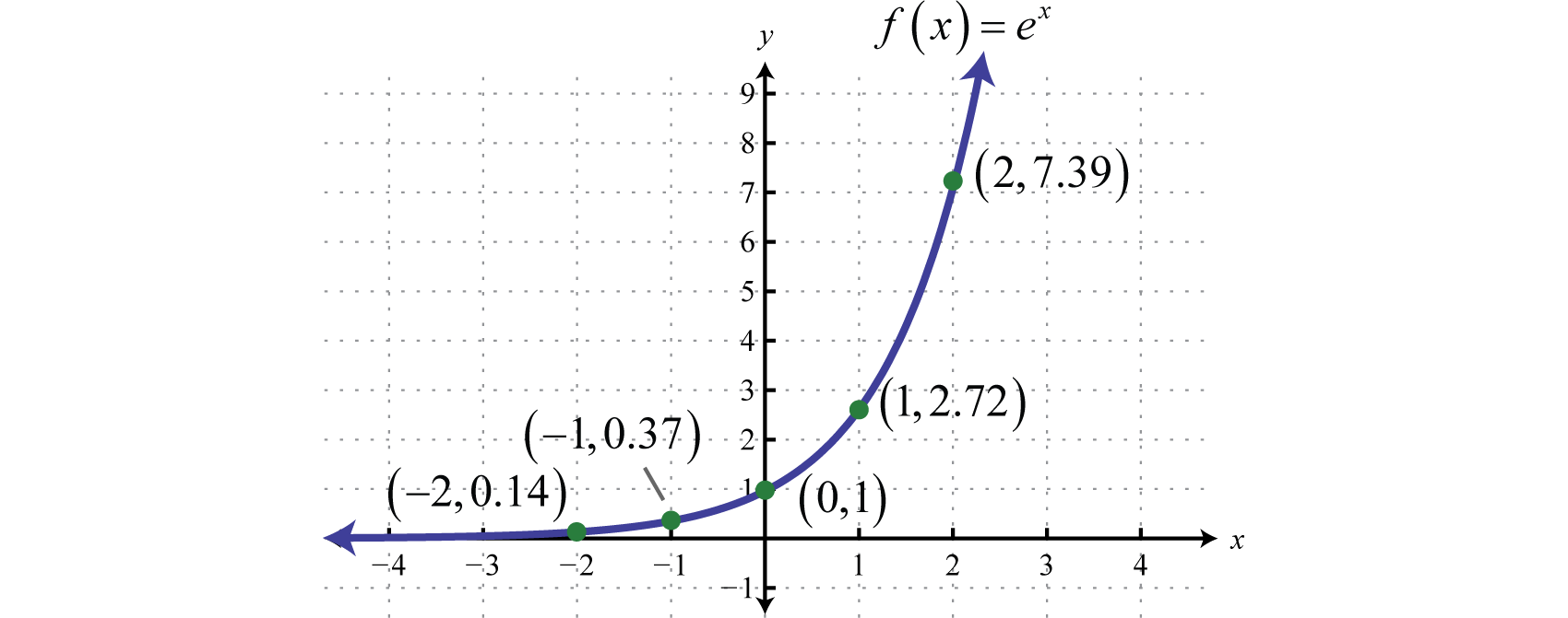
# (xenc @ W) are interpreted as +ve and -ve, but instead we'll interpret them as log counts and element-wise exponentiate these numbers
(xenc @ W).exp()tensor([[ 0.7881, 1.4508, 0.5454, 1.3093, 0.6097, 0.8072, 1.4556, 0.3797,
0.7659, 0.5242, 2.5262, 3.9600, 0.6496, 1.4932, 0.5022, 0.5264,
3.7490, 0.9699, 2.9359, 2.5183, 2.1339, 0.7493, 0.5667, 1.2279,
0.3848, 0.8546, 1.1020],
[ 3.4824, 0.5229, 18.9670, 0.3176, 0.5677, 1.3210, 0.3993, 6.5021,
0.3459, 0.6327, 4.6447, 1.1357, 1.1237, 0.9261, 2.1973, 1.3926,
0.9642, 1.5906, 0.6921, 1.0947, 1.5124, 0.5128, 1.1955, 0.5095,
0.8418, 2.4459, 2.1527],
[ 0.7579, 0.3810, 0.1629, 2.5622, 2.5319, 0.3934, 1.5204, 1.2851,
2.6746, 3.1084, 0.9689, 0.3935, 1.3860, 0.3209, 0.3803, 4.9112,
2.1981, 1.2541, 2.3506, 0.0639, 7.5321, 0.3261, 0.1782, 0.8298,
1.1250, 0.4843, 1.6050],
[ 0.7579, 0.3810, 0.1629, 2.5622, 2.5319, 0.3934, 1.5204, 1.2851,
2.6746, 3.1084, 0.9689, 0.3935, 1.3860, 0.3209, 0.3803, 4.9112,
2.1981, 1.2541, 2.3506, 0.0639, 7.5321, 0.3261, 0.1782, 0.8298,
1.1250, 0.4843, 1.6050],
[ 0.8150, 0.8897, 0.5635, 0.5420, 0.3049, 4.7245, 1.4128, 0.3884,
0.8230, 2.0519, 0.3190, 1.8373, 1.8544, 4.2920, 0.6231, 0.2958,
1.8875, 1.6357, 3.0929, 0.1260, 0.9692, 5.5058, 0.2598, 1.2371,
0.3233, 0.3116, 0.1762]])# note that all -ve nums turned to 0-1 and all +ve nums are >1.
# these exponentiated outputs can be interpreted (unlike prev -ve, +ve nums) like counts in our earlier matrix example
# so these values are >0 and take values based on settings of W. hmm nicelogits = xenc @ W # also referred to as logits or log counts
counts = logits.exp() # equivalent to the N matrix we previously built(that 2d array where each element's value was count for next character given a current character)
# normalize the rows of our count matrix to get the probability distribution
# sum along the first dimension
probs = counts / counts.sum(1, keepdims=True)
probstensor([[0.0222, 0.0409, 0.0154, 0.0369, 0.0172, 0.0227, 0.0410, 0.0107, 0.0216,
0.0148, 0.0712, 0.1116, 0.0183, 0.0421, 0.0142, 0.0148, 0.1056, 0.0273,
0.0827, 0.0710, 0.0601, 0.0211, 0.0160, 0.0346, 0.0108, 0.0241, 0.0311],
[0.0601, 0.0090, 0.3271, 0.0055, 0.0098, 0.0228, 0.0069, 0.1121, 0.0060,
0.0109, 0.0801, 0.0196, 0.0194, 0.0160, 0.0379, 0.0240, 0.0166, 0.0274,
0.0119, 0.0189, 0.0261, 0.0088, 0.0206, 0.0088, 0.0145, 0.0422, 0.0371],
[0.0182, 0.0091, 0.0039, 0.0615, 0.0607, 0.0094, 0.0365, 0.0308, 0.0642,
0.0746, 0.0232, 0.0094, 0.0333, 0.0077, 0.0091, 0.1178, 0.0527, 0.0301,
0.0564, 0.0015, 0.1807, 0.0078, 0.0043, 0.0199, 0.0270, 0.0116, 0.0385],
[0.0182, 0.0091, 0.0039, 0.0615, 0.0607, 0.0094, 0.0365, 0.0308, 0.0642,
0.0746, 0.0232, 0.0094, 0.0333, 0.0077, 0.0091, 0.1178, 0.0527, 0.0301,
0.0564, 0.0015, 0.1807, 0.0078, 0.0043, 0.0199, 0.0270, 0.0116, 0.0385],
[0.0219, 0.0239, 0.0151, 0.0145, 0.0082, 0.1268, 0.0379, 0.0104, 0.0221,
0.0551, 0.0086, 0.0493, 0.0498, 0.1152, 0.0167, 0.0079, 0.0507, 0.0439,
0.0830, 0.0034, 0.0260, 0.1478, 0.0070, 0.0332, 0.0087, 0.0084, 0.0047]])probs[3].sum() # every row sums to one cuz they're normalizedtensor(1.)probs.shapetorch.Size([5, 27])# what did we achieve?
# note: by 5 examples: we mean 1 word emma: eg 1: .e, eg2: em, eg3: mm, eg4: ma, eg5: a.
# for every single one of our 5 examples, we have a row that came out of a neural net, and because of the transformations, we ensure the outputs are probabilities# logits = xenc @ W #wx
# counts = logits.exp()
# probs = counts / counts.sum(1, keepdims=True)
# all three operations above are differentiable, and we can backpropagate through them, and we get probability distributions# for the zeroth example, where we fed in .e of emma. we input a . and expect a e as output with high probability
# we first had one_hot vector of zeroth example, i.e. we fed the dot into a neural net
# it went into the neural net and produced a probability distribution: probs[0]probs[0]
# this distribution tells us how likely each of the 27 characters are to come after first character "."
# then as we tune our weights, we will get different probabilities
# now the qn is: how to optimize and get good weights? so that the probability distribution coming out is good
# and how we measure the goodness: is by LOSS FUNCTIONtensor([0.0222, 0.0409, 0.0154, 0.0369, 0.0172, 0.0227, 0.0410, 0.0107, 0.0216,
0.0148, 0.0712, 0.1116, 0.0183, 0.0421, 0.0142, 0.0148, 0.1056, 0.0273,
0.0827, 0.0710, 0.0601, 0.0211, 0.0160, 0.0346, 0.0108, 0.0241, 0.0311])probs[0].sum()tensor(1.)probs[0].shapetorch.Size([27])# continue from 1:26:24# SUMMARY---------------------------------------------------------------------------------------------------------------------------------------print(xs)
print(ys) # labels for the correct next character in the sequencetensor([ 0, 5, 13, 13, 1])
tensor([ 5, 13, 13, 1, 0])
# randomly initialize 27 neuron's weights. Each neuron receives 27 inputs
g = torch.Generator().manual_seed(2147483647)
W = torch.randn((27, 27), generator=g)# FORWARD PASS# input to the network: one-hot encoding
xenc = F.one_hot(xs, num_classes = 27).float() # AN ARRAY OF 5X27
# predict log-counts
logits = xenc @ W
# Note: The following two lines of code together is called a 'softmax'
# counts: equivalent to N
counts = logits.exp()
# probabilities for next character
probs = counts/counts.sum(1, keepdims=True)probs.shapetorch.Size([5, 27])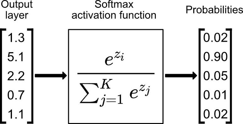
Softmax and loss
# softmax: often used layer in neural net that takes input z(a vector of logits, i.e. raw neural network outputs) into a probability distribution
# It exponentiates each logit and then normalizes by dividing by the sum
# of all exponentiated values.
# Input: any real numbers (positive, negative, or zero).
# Before normalization:
# - negative logits become numbers between 0 and 1 after exponentiation
# - zero becomes 1
# - positive logits become numbers greater than 1
# Output:
# - all values are positive
# - all values sum to 1
# - each value represents the probability of that class
# Softmax is commonly used as the final layer of a classifier to convert
# logits into class probabilities.# Note: that in the above forward pass, everything is made up of differentiable layers
# we can backpropagate through everything there, eg. matrix multiplication is just multiplication and addition, exponentiation(can be backpropagated through)
# also sum and division are backpropagatablenlls = torch.zeros(5) #since we have five bigrams that make up emma: .e, em, mm, ma, a.
for i in range(5):
# i-th bigram:
x = xs[i].item() #input character index
y = ys[i].item() #label character index
print('--------')
print(f'bigram example {i+1}: {itos[x]}{itos[y]} (indexes {x},{y})')
print('input to the neural net:', x)
print('output probabilities from the neural net:', probs[i])
print('label (actual next character):', y)
# what probability the forward pass actually gave us for our label character(will probably be less than expected)
p = probs[i, y]#the model thinks that e following ., i.e. e being the first char is 1% likely, which is not very good
print('probability assigned by the neural net to the correct character:', p.item())
logp = torch.log(p)
print('log likelihood:', logp.item())
nll = -logp
print('negative log likelihood:', nll.item()) #4.3 is very high, and we will get a very big loss initially which is not good
nlls[i] = nll
print('======')
print('average negative log likelihood, i.e. loss=', nlls.mean().item())
# you can try changing the W, resample and with different seed, you might get better W
# but this hit and trial approach for optimization is a noob way, you should just use backprop and train the model to do better--------
bigram example 1: .e (indexes 0,5)
input to the neural net: 0
output probabilities from the neural net: tensor([0.0607, 0.0100, 0.0123, 0.0042, 0.0168, 0.0123, 0.0027, 0.0232, 0.0137,
0.0313, 0.0079, 0.0278, 0.0091, 0.0082, 0.0500, 0.2378, 0.0603, 0.0025,
0.0249, 0.0055, 0.0339, 0.0109, 0.0029, 0.0198, 0.0118, 0.1537, 0.1459])
label (actual next character): 5
probability assigned by the neural net to the correct character: 0.01228625513613224
log likelihood: -4.399273872375488
negative log likelihood: 4.399273872375488
--------
bigram example 2: em (indexes 5,13)
input to the neural net: 5
output probabilities from the neural net: tensor([0.0290, 0.0796, 0.0248, 0.0521, 0.1989, 0.0289, 0.0094, 0.0335, 0.0097,
0.0301, 0.0702, 0.0228, 0.0115, 0.0181, 0.0108, 0.0315, 0.0291, 0.0045,
0.0916, 0.0215, 0.0486, 0.0300, 0.0501, 0.0027, 0.0118, 0.0022, 0.0472])
label (actual next character): 13
probability assigned by the neural net to the correct character: 0.018050700426101685
log likelihood: -4.014570713043213
negative log likelihood: 4.014570713043213
--------
bigram example 3: mm (indexes 13,13)
input to the neural net: 13
output probabilities from the neural net: tensor([0.0312, 0.0737, 0.0484, 0.0333, 0.0674, 0.0200, 0.0263, 0.0249, 0.1226,
0.0164, 0.0075, 0.0789, 0.0131, 0.0267, 0.0147, 0.0112, 0.0585, 0.0121,
0.0650, 0.0058, 0.0208, 0.0078, 0.0133, 0.0203, 0.1204, 0.0469, 0.0126])
label (actual next character): 13
probability assigned by the neural net to the correct character: 0.026691533625125885
log likelihood: -3.623408794403076
negative log likelihood: 3.623408794403076
--------
bigram example 4: ma (indexes 13,1)
input to the neural net: 13
output probabilities from the neural net: tensor([0.0312, 0.0737, 0.0484, 0.0333, 0.0674, 0.0200, 0.0263, 0.0249, 0.1226,
0.0164, 0.0075, 0.0789, 0.0131, 0.0267, 0.0147, 0.0112, 0.0585, 0.0121,
0.0650, 0.0058, 0.0208, 0.0078, 0.0133, 0.0203, 0.1204, 0.0469, 0.0126])
label (actual next character): 1
probability assigned by the neural net to the correct character: 0.07367686182260513
log likelihood: -2.6080665588378906
negative log likelihood: 2.6080665588378906
--------
bigram example 5: a. (indexes 1,0)
input to the neural net: 1
output probabilities from the neural net: tensor([0.0150, 0.0086, 0.0396, 0.0100, 0.0606, 0.0308, 0.1084, 0.0131, 0.0125,
0.0048, 0.1024, 0.0086, 0.0988, 0.0112, 0.0232, 0.0207, 0.0408, 0.0078,
0.0899, 0.0531, 0.0463, 0.0309, 0.0051, 0.0329, 0.0654, 0.0503, 0.0091])
label (actual next character): 0
probability assigned by the neural net to the correct character: 0.014977526850998402
log likelihood: -4.201204299926758
negative log likelihood: 4.201204299926758
======
average negative log likelihood, i.e. loss= 3.7693049907684326
# we have a loss function: nlls.mean().item()
# and this is made up of only differentiable operations
# and we can minimize loss but tuning the W(weights) by computing the gradients of the loss w.r.t W matrices, i.e. gradient-based optimization# what we'll do is very similar to what we did in micrograd
# in micrograd we had four input examples and their targets
# xs = [
# [2.0, 3.0, -1.0],
# [3.0, -1.0, 0.5],
# [0.5, 1.0, 1.0],
# [1.0, 1.0, -1.0]
# ]
# ys = [1.0, -1.0, -1.0, 1.0] # desired targets,
# but our input has xs as tensor([0, 5, 13, 13, 1]) which can be converted to one_hot and be 5x27 just like xs above
# but we won't have a desired ys,
# instead we will try to minimize our loss upto the point that it is similar to the loss computed from earlier method 1: table approach# in micrograd, our neural net was n(x) which was a multi layer perceptron
# say we want input layer with 3 neurons, 2 hidden layers each having four neurons and an output unit
# x = [2.0, 3.0, -1.0]
# n = MLP(3, [4, 4, 1])# we want 3 inputs into 2 layers of 4 and one output
# n(x)# but our neural net is just a single linear layer of matrix multiplication(wx) which is followed by a softmax
# our neural network: logits = xenc @ W, followed by 2 lines of softmax# in micrograd, loss was mean square error, we just subtracted prediction from ground truth, then squared it and summed it all up
# ypred = [n(x) for x in xs]
# loss = sum([(ygt - yout)**2 for ygt, yout in zip(ys, ypred)])
# here, loss=single num that represented the quality of neural net, and when loss is low, it showed that the neural net was predicting correctly
# then we iterated over all parameters, and set gradient to zero
# and called loss.backward
# backward pass
# for p in n.parameters():
# p.grad = 0.0
# loss.backward() #initiated backpropagation at final output node of loss, i.e. just filled the gradients that were recently reset to 0
# and during backpropagation, we updated/nudged all the parameters slightly in the negative direction of gradient, i.e. tuning weights, i.e. training
# update: gradient descent
# for p in n.parameters():
# p.data += (-0.05) * p.grad# we're going to do the same thing here too
# here, probs is our ypred
# to evaluate loss: we don't use MSE, we have negative log likelihood cuz in this case we're doing classification(not regression like in micrograd)# first of all, we want to be able to pluck out the probabilities at correct indices from probs
probs.shapetorch.Size([5, 27])print(xs)
print(ys)tensor([ 0, 5, 13, 13, 1])
tensor([ 5, 13, 13, 1, 0])
probstensor([[0.0607, 0.0100, 0.0123, 0.0042, 0.0168, 0.0123, 0.0027, 0.0232, 0.0137,
0.0313, 0.0079, 0.0278, 0.0091, 0.0082, 0.0500, 0.2378, 0.0603, 0.0025,
0.0249, 0.0055, 0.0339, 0.0109, 0.0029, 0.0198, 0.0118, 0.1537, 0.1459],
[0.0290, 0.0796, 0.0248, 0.0521, 0.1989, 0.0289, 0.0094, 0.0335, 0.0097,
0.0301, 0.0702, 0.0228, 0.0115, 0.0181, 0.0108, 0.0315, 0.0291, 0.0045,
0.0916, 0.0215, 0.0486, 0.0300, 0.0501, 0.0027, 0.0118, 0.0022, 0.0472],
[0.0312, 0.0737, 0.0484, 0.0333, 0.0674, 0.0200, 0.0263, 0.0249, 0.1226,
0.0164, 0.0075, 0.0789, 0.0131, 0.0267, 0.0147, 0.0112, 0.0585, 0.0121,
0.0650, 0.0058, 0.0208, 0.0078, 0.0133, 0.0203, 0.1204, 0.0469, 0.0126],
[0.0312, 0.0737, 0.0484, 0.0333, 0.0674, 0.0200, 0.0263, 0.0249, 0.1226,
0.0164, 0.0075, 0.0789, 0.0131, 0.0267, 0.0147, 0.0112, 0.0585, 0.0121,
0.0650, 0.0058, 0.0208, 0.0078, 0.0133, 0.0203, 0.1204, 0.0469, 0.0126],
[0.0150, 0.0086, 0.0396, 0.0100, 0.0606, 0.0308, 0.1084, 0.0131, 0.0125,
0.0048, 0.1024, 0.0086, 0.0988, 0.0112, 0.0232, 0.0207, 0.0408, 0.0078,
0.0899, 0.0531, 0.0463, 0.0309, 0.0051, 0.0329, 0.0654, 0.0503, 0.0091]])# eg. to get the probs of labels(ys) for 5 bigrams
# probs[0,5]: how likely are we to get 5(e) given that we have a 0(.)
# probs[1, 13]: how likely are we to get 13(m) given that we have a 5(e)
# probs[2, 13]: how likely are we to get 13(m) given that we have a 13(m)
# probs[3, 1]: how likely are we to get 1(a) given that we have a 13(m)
# probs[4, 0]: how likely are we to get 0(.) given that we have a 1(a)
# don't get confused by use of 0-4, 0th row is first bigram, 1st row is 2nd bigram, and each entry gives prob for next char
probs[0, 5], probs[1, 13], probs[2,13], probs[3, 1], probs[4, 0](tensor(0.0123),
tensor(0.0181),
tensor(0.0267),
tensor(0.0737),
tensor(0.0150))print(torch.arange(0,5))
print(ys)tensor([0, 1, 2, 3, 4])
tensor([ 5, 13, 13, 1, 0])
# we want a more efficient way to access these probabilities instead of listing them out in a tuple
# one alternative in pytorch: we can pass all these integers in a vector
probs[torch.arange(5), ys]tensor([0.0123, 0.0181, 0.0267, 0.0737, 0.0150])# so we plucked out the probabilities assigned by the neural network to the correct next characters for 5 bigrams we're working with# now, we look at the log probabilities
print(probs[torch.arange(5), ys].log())
# then we want avg
print(probs[torch.arange(5), ys].log().mean())
# now add -ve sign to get -ve avg log likelihood: which is our loss
loss = -probs[torch.arange(5), ys].log().mean()
losstensor([-4.3993, -4.0146, -3.6234, -2.6081, -4.2012])
tensor(-3.7693)
tensor(3.7693)# note: this loss matches the loss we obtained above(but this is a vectorized form)
# average negative log likelihood, i.e. loss= 3.7693049907684326# so, we defined our forward pass: we have our probs(ypred) and loss
# now, we do backward passGradient-based learning
# backward pass
# 1. make sure all gradients are reset: 0
# in pytorch, we can set all gradients to zero or None
# setting gradients to None: more efficient as it is interpreted as lack of gradient, and same as zeros too
# then we do loss.backward, but remember that pytorch requires we pass in requires_grad=True while generating the random weights initially# randomly initialize 27 neuron's weights. Each neuron receives 27 inputs
g = torch.Generator().manual_seed(2147483647)
W = torch.randn((27, 27), generator=g, requires_grad=True)# forward pass
xenc = F.one_hot(xs, num_classes = 27).float() # AN ARRAY OF 5X27
logits = xenc @ W
counts = logits.exp()
probs = counts/counts.sum(1, keepdims=True)
loss = -probs[torch.arange(5), ys].log().mean()# backward pass
W.grad = None #set zero to the gradient
loss.backward()# in our forward pass above, pytorch actually keeps track of all the operations we did under the hood and builds a full computational graph
# those graphs exist inside pytorch, it knows all the dependencies and all the mathematical operations
# this loss.backward() just fills in the gradients of all the intermediates all the way back to W(parameters of our neural net)print(W.shape)
print(W.grad.shape)torch.Size([27, 27])
torch.Size([27, 27])
# so, W[0,0] = 0.0121 is +ve
# it tells us that slightly increasing it will increase the loss: eg. W[0,0] += h# every element of W.grad tells us the influence of that weight on the loss function
W.gradtensor([[ 0.0121, 0.0020, 0.0025, 0.0008, 0.0034, -0.1975, 0.0005, 0.0046,
0.0027, 0.0063, 0.0016, 0.0056, 0.0018, 0.0016, 0.0100, 0.0476,
0.0121, 0.0005, 0.0050, 0.0011, 0.0068, 0.0022, 0.0006, 0.0040,
0.0024, 0.0307, 0.0292],
[-0.1970, 0.0017, 0.0079, 0.0020, 0.0121, 0.0062, 0.0217, 0.0026,
0.0025, 0.0010, 0.0205, 0.0017, 0.0198, 0.0022, 0.0046, 0.0041,
0.0082, 0.0016, 0.0180, 0.0106, 0.0093, 0.0062, 0.0010, 0.0066,
0.0131, 0.0101, 0.0018],
[ 0.0000, 0.0000, 0.0000, 0.0000, 0.0000, 0.0000, 0.0000, 0.0000,
0.0000, 0.0000, 0.0000, 0.0000, 0.0000, 0.0000, 0.0000, 0.0000,
0.0000, 0.0000, 0.0000, 0.0000, 0.0000, 0.0000, 0.0000, 0.0000,
0.0000, 0.0000, 0.0000],
[ 0.0000, 0.0000, 0.0000, 0.0000, 0.0000, 0.0000, 0.0000, 0.0000,
0.0000, 0.0000, 0.0000, 0.0000, 0.0000, 0.0000, 0.0000, 0.0000,
0.0000, 0.0000, 0.0000, 0.0000, 0.0000, 0.0000, 0.0000, 0.0000,
0.0000, 0.0000, 0.0000],
[ 0.0000, 0.0000, 0.0000, 0.0000, 0.0000, 0.0000, 0.0000, 0.0000,
0.0000, 0.0000, 0.0000, 0.0000, 0.0000, 0.0000, 0.0000, 0.0000,
0.0000, 0.0000, 0.0000, 0.0000, 0.0000, 0.0000, 0.0000, 0.0000,
0.0000, 0.0000, 0.0000],
[ 0.0058, 0.0159, 0.0050, 0.0104, 0.0398, 0.0058, 0.0019, 0.0067,
0.0019, 0.0060, 0.0140, 0.0046, 0.0023, -0.1964, 0.0022, 0.0063,
0.0058, 0.0009, 0.0183, 0.0043, 0.0097, 0.0060, 0.0100, 0.0005,
0.0024, 0.0004, 0.0094],
[ 0.0000, 0.0000, 0.0000, 0.0000, 0.0000, 0.0000, 0.0000, 0.0000,
0.0000, 0.0000, 0.0000, 0.0000, 0.0000, 0.0000, 0.0000, 0.0000,
0.0000, 0.0000, 0.0000, 0.0000, 0.0000, 0.0000, 0.0000, 0.0000,
0.0000, 0.0000, 0.0000],
[ 0.0000, 0.0000, 0.0000, 0.0000, 0.0000, 0.0000, 0.0000, 0.0000,
0.0000, 0.0000, 0.0000, 0.0000, 0.0000, 0.0000, 0.0000, 0.0000,
0.0000, 0.0000, 0.0000, 0.0000, 0.0000, 0.0000, 0.0000, 0.0000,
0.0000, 0.0000, 0.0000],
[ 0.0000, 0.0000, 0.0000, 0.0000, 0.0000, 0.0000, 0.0000, 0.0000,
0.0000, 0.0000, 0.0000, 0.0000, 0.0000, 0.0000, 0.0000, 0.0000,
0.0000, 0.0000, 0.0000, 0.0000, 0.0000, 0.0000, 0.0000, 0.0000,
0.0000, 0.0000, 0.0000],
[ 0.0000, 0.0000, 0.0000, 0.0000, 0.0000, 0.0000, 0.0000, 0.0000,
0.0000, 0.0000, 0.0000, 0.0000, 0.0000, 0.0000, 0.0000, 0.0000,
0.0000, 0.0000, 0.0000, 0.0000, 0.0000, 0.0000, 0.0000, 0.0000,
0.0000, 0.0000, 0.0000],
[ 0.0000, 0.0000, 0.0000, 0.0000, 0.0000, 0.0000, 0.0000, 0.0000,
0.0000, 0.0000, 0.0000, 0.0000, 0.0000, 0.0000, 0.0000, 0.0000,
0.0000, 0.0000, 0.0000, 0.0000, 0.0000, 0.0000, 0.0000, 0.0000,
0.0000, 0.0000, 0.0000],
[ 0.0000, 0.0000, 0.0000, 0.0000, 0.0000, 0.0000, 0.0000, 0.0000,
0.0000, 0.0000, 0.0000, 0.0000, 0.0000, 0.0000, 0.0000, 0.0000,
0.0000, 0.0000, 0.0000, 0.0000, 0.0000, 0.0000, 0.0000, 0.0000,
0.0000, 0.0000, 0.0000],
[ 0.0000, 0.0000, 0.0000, 0.0000, 0.0000, 0.0000, 0.0000, 0.0000,
0.0000, 0.0000, 0.0000, 0.0000, 0.0000, 0.0000, 0.0000, 0.0000,
0.0000, 0.0000, 0.0000, 0.0000, 0.0000, 0.0000, 0.0000, 0.0000,
0.0000, 0.0000, 0.0000],
[ 0.0125, -0.1705, 0.0194, 0.0133, 0.0270, 0.0080, 0.0105, 0.0100,
0.0490, 0.0066, 0.0030, 0.0316, 0.0052, -0.1893, 0.0059, 0.0045,
0.0234, 0.0049, 0.0260, 0.0023, 0.0083, 0.0031, 0.0053, 0.0081,
0.0482, 0.0187, 0.0051],
[ 0.0000, 0.0000, 0.0000, 0.0000, 0.0000, 0.0000, 0.0000, 0.0000,
0.0000, 0.0000, 0.0000, 0.0000, 0.0000, 0.0000, 0.0000, 0.0000,
0.0000, 0.0000, 0.0000, 0.0000, 0.0000, 0.0000, 0.0000, 0.0000,
0.0000, 0.0000, 0.0000],
[ 0.0000, 0.0000, 0.0000, 0.0000, 0.0000, 0.0000, 0.0000, 0.0000,
0.0000, 0.0000, 0.0000, 0.0000, 0.0000, 0.0000, 0.0000, 0.0000,
0.0000, 0.0000, 0.0000, 0.0000, 0.0000, 0.0000, 0.0000, 0.0000,
0.0000, 0.0000, 0.0000],
[ 0.0000, 0.0000, 0.0000, 0.0000, 0.0000, 0.0000, 0.0000, 0.0000,
0.0000, 0.0000, 0.0000, 0.0000, 0.0000, 0.0000, 0.0000, 0.0000,
0.0000, 0.0000, 0.0000, 0.0000, 0.0000, 0.0000, 0.0000, 0.0000,
0.0000, 0.0000, 0.0000],
[ 0.0000, 0.0000, 0.0000, 0.0000, 0.0000, 0.0000, 0.0000, 0.0000,
0.0000, 0.0000, 0.0000, 0.0000, 0.0000, 0.0000, 0.0000, 0.0000,
0.0000, 0.0000, 0.0000, 0.0000, 0.0000, 0.0000, 0.0000, 0.0000,
0.0000, 0.0000, 0.0000],
[ 0.0000, 0.0000, 0.0000, 0.0000, 0.0000, 0.0000, 0.0000, 0.0000,
0.0000, 0.0000, 0.0000, 0.0000, 0.0000, 0.0000, 0.0000, 0.0000,
0.0000, 0.0000, 0.0000, 0.0000, 0.0000, 0.0000, 0.0000, 0.0000,
0.0000, 0.0000, 0.0000],
[ 0.0000, 0.0000, 0.0000, 0.0000, 0.0000, 0.0000, 0.0000, 0.0000,
0.0000, 0.0000, 0.0000, 0.0000, 0.0000, 0.0000, 0.0000, 0.0000,
0.0000, 0.0000, 0.0000, 0.0000, 0.0000, 0.0000, 0.0000, 0.0000,
0.0000, 0.0000, 0.0000],
[ 0.0000, 0.0000, 0.0000, 0.0000, 0.0000, 0.0000, 0.0000, 0.0000,
0.0000, 0.0000, 0.0000, 0.0000, 0.0000, 0.0000, 0.0000, 0.0000,
0.0000, 0.0000, 0.0000, 0.0000, 0.0000, 0.0000, 0.0000, 0.0000,
0.0000, 0.0000, 0.0000],
[ 0.0000, 0.0000, 0.0000, 0.0000, 0.0000, 0.0000, 0.0000, 0.0000,
0.0000, 0.0000, 0.0000, 0.0000, 0.0000, 0.0000, 0.0000, 0.0000,
0.0000, 0.0000, 0.0000, 0.0000, 0.0000, 0.0000, 0.0000, 0.0000,
0.0000, 0.0000, 0.0000],
[ 0.0000, 0.0000, 0.0000, 0.0000, 0.0000, 0.0000, 0.0000, 0.0000,
0.0000, 0.0000, 0.0000, 0.0000, 0.0000, 0.0000, 0.0000, 0.0000,
0.0000, 0.0000, 0.0000, 0.0000, 0.0000, 0.0000, 0.0000, 0.0000,
0.0000, 0.0000, 0.0000],
[ 0.0000, 0.0000, 0.0000, 0.0000, 0.0000, 0.0000, 0.0000, 0.0000,
0.0000, 0.0000, 0.0000, 0.0000, 0.0000, 0.0000, 0.0000, 0.0000,
0.0000, 0.0000, 0.0000, 0.0000, 0.0000, 0.0000, 0.0000, 0.0000,
0.0000, 0.0000, 0.0000],
[ 0.0000, 0.0000, 0.0000, 0.0000, 0.0000, 0.0000, 0.0000, 0.0000,
0.0000, 0.0000, 0.0000, 0.0000, 0.0000, 0.0000, 0.0000, 0.0000,
0.0000, 0.0000, 0.0000, 0.0000, 0.0000, 0.0000, 0.0000, 0.0000,
0.0000, 0.0000, 0.0000],
[ 0.0000, 0.0000, 0.0000, 0.0000, 0.0000, 0.0000, 0.0000, 0.0000,
0.0000, 0.0000, 0.0000, 0.0000, 0.0000, 0.0000, 0.0000, 0.0000,
0.0000, 0.0000, 0.0000, 0.0000, 0.0000, 0.0000, 0.0000, 0.0000,
0.0000, 0.0000, 0.0000],
[ 0.0000, 0.0000, 0.0000, 0.0000, 0.0000, 0.0000, 0.0000, 0.0000,
0.0000, 0.0000, 0.0000, 0.0000, 0.0000, 0.0000, 0.0000, 0.0000,
0.0000, 0.0000, 0.0000, 0.0000, 0.0000, 0.0000, 0.0000, 0.0000,
0.0000, 0.0000, 0.0000]])# we use this gradient information to update the weights of our neural network
# we don't need to loop over all parameters like in micrograd as for p in p.parameters()
# because we only have one parameter tensor: W
# so we can simply run this one line instead to update our tensor weights
W.data += -0.1 * W.grad# so now, we expect that the loss should have decreased
print(loss.item())3.7693049907684326
# run cell of forward pass then backward pass again and again manually to see loss decreasing, or you could just use loop# forward pass
xenc = F.one_hot(xs, num_classes = 27).float() # AN ARRAY OF 5X27
logits = xenc @ W
counts = logits.exp()
probs = counts/counts.sum(1, keepdims=True)
loss = -probs[torch.arange(5), ys].log().mean()
# backward pass
W.grad = None #set zero to the gradient
loss.backward()
W.data += -0.1 * W.grad
print(loss.item())3.6690573692321777
# the process of gradient descent
for i in range(15):
# forward pass
xenc = F.one_hot(xs, num_classes = 27).float() # AN ARRAY OF 5X27
logits = xenc @ W
counts = logits.exp()
probs = counts/counts.sum(1, keepdims=True)
loss = -probs[torch.arange(5), ys].log().mean()
# backward pass
W.grad = None #set zero to the gradient
loss.backward()
W.data += -0.1 * W.grad
print(loss.item())3.649179458618164
3.629345655441284
3.609556198120117
3.589811325073242
3.5701117515563965
3.5504581928253174
3.530850648880005
3.5112900733947754
3.49177622795105
3.4723105430603027
3.452892303466797
3.433523178100586
3.4142024517059326
3.3949317932128906
3.3757102489471436
# getting lower loss: equivalent to: neural network is assigning high probabilities to the correct next characters# rearranged everything and put together------------------------FROM START-------------------------------------------------------xs, ys = [], []
# for w in words[:1]:
for w in words:
chs = ['.'] + list(w) + ['.']
for ch1, ch2 in zip(chs, chs[1:]):
ix1 = stoi[ch1]
ix2 = stoi[ch2]
xs.append(ix1)
ys.append(ix2)
xs = torch.tensor(xs)
ys = torch.tensor(ys)
num = xs.nelement()
print("total number of examples/bigrams:", num)
# initialize the network
g = torch.Generator().manual_seed(2147483647)
W = torch.randn((27, 27), generator = g, requires_grad=True)total number of examples/bigrams: 228146
Comparing counts with learning
# what number do we expect to be our desired loss?
# we expect something we got originally when we had optimized just by counting, our loss was roughly 2.47 after smoothing
# getting approximately 2.46 is the goal, and not down to 0.0003, but why?
# because we're not taking any additional information, we're just taking the previous character and trying to predict the next one
# but instead of trying to do it by explicit counting and normalizing, we're doing it with gradient based learning
# this gradient based approach is way more flexible and scalable, we can now expand this approach and complexify the neural net
# currently we're just taking 1 char and predicting next char, but we can substantially/largely iterate on this
# eg. we take multiple previous characters instead of just 1, and feed it into very complex neural nets too
# but fundamentally, the output of the neural nets will just be logits, and the logits will go through the exact same transformation
# we'll take it through softmax, calculate the loss function and the negative log likelihood, and do gradient-based optimization# as we complexify the neural nets and work all the way upto transformers, the structure is the same fundamentally
# the only thing that will change/be more complex is the way we,
# the way we do the forward pass where we take the previous chars to calculate the logits for the next character# in our initial table based approach, it is not scalable, there'll be way too many combinations of what previous characters could be
# it works for 1char input, 1 char output, but doesn't work well for 10char input 1 char output, it was an unscalable approach
# but our neural network approach is very scalable and flexible too# the process of gradient descent
for i in range(200):
# forward pass
xenc = F.one_hot(xs, num_classes = 27).float() # AN ARRAY OF numX27
logits = xenc @ W
counts = logits.exp()
probs = counts/counts.sum(1, keepdims=True)
loss = -probs[torch.arange(num), ys].log().mean()
# backward pass
W.grad = None #set zero to the gradient
loss.backward()
W.data += -50 * W.grad
print(loss.item())3.758953332901001
3.371100664138794
3.1540427207946777
3.020374059677124
2.927711248397827
2.8604023456573486
2.8097290992736816
2.7701022624969482
2.7380728721618652
2.711496353149414
2.6890032291412354
2.6696884632110596
2.6529300212860107
2.638277292251587
2.6253879070281982
2.613990545272827
2.60386323928833
2.5948219299316406
2.5867116451263428
2.5794036388397217
2.572789192199707
2.5667760372161865
2.5612878799438477
2.5562589168548584
2.551633596420288
2.547365665435791
2.5434155464172363
2.5397486686706543
2.5363364219665527
2.533154249191284
2.5301806926727295
2.5273969173431396
2.5247862339019775
2.522334575653076
2.520028829574585
2.5178580284118652
2.515810489654541
2.513878107070923
2.512052059173584
2.510324001312256
2.5086872577667236
2.5071349143981934
2.5056610107421875
2.504261016845703
2.502929210662842
2.5016608238220215
2.5004520416259766
2.4992988109588623
2.498197317123413
2.497144937515259
2.496137857437134
2.495173692703247
2.4942493438720703
2.49336314201355
2.4925124645233154
2.4916954040527344
2.4909095764160156
2.4901537895202637
2.4894261360168457
2.488725423812866
2.488049268722534
2.4873974323272705
2.4867680072784424
2.4861602783203125
2.4855728149414062
2.4850046634674072
2.484455108642578
2.4839231967926025
2.483408212661743
2.4829084873199463
2.482424259185791
2.48195481300354
2.481499195098877
2.4810571670532227
2.4806275367736816
2.480210065841675
2.479804515838623
2.479410409927368
2.4790267944335938
2.4786536693573
2.478290557861328
2.4779367446899414
2.4775924682617188
2.477257251739502
2.4769303798675537
2.476611852645874
2.4763007164001465
2.4759979248046875
2.4757025241851807
2.475414276123047
2.475132703781128
2.474858045578003
2.4745898246765137
2.474327564239502
2.474071979522705
2.4738216400146484
2.4735772609710693
2.4733383655548096
2.47310471534729
2.4728758335113525
2.4726529121398926
2.4724340438842773
2.4722201824188232
2.472010850906372
2.4718058109283447
2.4716053009033203
2.471409320831299
2.471216917037964
2.4710283279418945
2.470843553543091
2.4706625938415527
2.4704854488372803
2.4703118801116943
2.4701414108276367
2.4699742794036865
2.4698104858398438
2.4696500301361084
2.469492197036743
2.4693377017974854
2.4691858291625977
2.4690372943878174
2.468891143798828
2.468747615814209
2.46860671043396
2.468468427658081
2.468332529067993
2.4681990146636963
2.4680681228637695
2.4679393768310547
2.4678127765655518
2.46768856048584
2.4675662517547607
2.4674463272094727
2.467327833175659
2.467211961746216
2.467097759246826
2.4669857025146484
2.4668753147125244
2.466766357421875
2.4666597843170166
2.466554641723633
2.4664509296417236
2.4663491249084473
2.4662492275238037
2.4661505222320557
2.4660532474517822
2.4659576416015625
2.4658634662628174
2.4657704830169678
2.465679407119751
2.4655895233154297
2.465500593185425
2.4654135704040527
2.465327501296997
2.465242624282837
2.4651591777801514
2.4650766849517822
2.4649956226348877
2.4649155139923096
2.464836597442627
2.46475887298584
2.464682102203369
2.464606285095215
2.464531660079956
2.4644579887390137
2.464385509490967
2.4643139839172363
2.464243173599243
2.4641737937927246
2.464104652404785
2.464036703109741
2.4639699459075928
2.4639039039611816
2.4638383388519287
2.463773727416992
2.463710308074951
2.4636473655700684
2.463585376739502
2.4635238647460938
2.463463306427002
2.4634037017822266
2.4633448123931885
2.4632863998413086
2.463228702545166
2.4631717205047607
2.463115692138672
2.463059902191162
2.4630050659179688
2.4629504680633545
2.4628970623016357
2.462843894958496
2.4627914428710938
2.462739944458008
2.462688684463501
2.4626379013061523
2.462587594985962
2.462538242340088
2.462489128112793
2.4624407291412354
2.462393045425415
# xenc is made up of one-hot vectors, and the one hot vectors are multiplied by the W matrix
# if we have a one-hot vector that eg. has a 1 at the fifth dimension, then because of the way matrix multiplication works
# multiplying that one-hot vector with W ends up plucking out the fifth row of W
# so logits would end up becoming the fifth row of W, cuz that's how matrix multiplication works
# like multiplying everything by 0 and just one entry by 1, it ends up copying that specific dimension,
# so it looks like logits just selects the row of the weight matrix
# logits = xenc @ W
print(xenc)tensor([[1., 0., 0., ..., 0., 0., 0.],
[0., 0., 0., ..., 0., 0., 0.],
[0., 0., 0., ..., 0., 0., 0.],
...,
[0., 0., 0., ..., 0., 1., 0.],
[0., 0., 0., ..., 0., 0., 1.],
[0., 0., 0., ..., 1., 0., 0.]])
# ahh ahh, remember that in the table method case where table=N, we used the first character to index the row of the array
# that row gave us the probability distribution for the next character
# i.e. first character was used as a lookup into matrix N to get probability distribution
# but what happens in neural network case is very similar too# we take the index by encoding xs as one-hot and multiplying it by W
# then logits becomes the row of W
# logits then gets exponentiated to create the counts then gets normalized and becomes probability
# so, W is almost the same as N, but W is the log counts, not the counts itself
# thus we can say W.exp = N table matrix
# N was filled by populating the counts of bigram
# but in gradient based framework, we initialized W randomly, then we let the loss guide us to arrive at the exact same array# qn: in this simple case we got loss from table case and used that to get loss for neural net.
# but what about other complex cases where we might not construct the table based on counts?# remember the smoothing in N case where we added fake count 1 to every entry to prevent probability from being 0 to any bigram
# but if we increase the count, probability becomes more and more uniformRegularization and sampling
# and interestingly, our gradient-based optimization of neural network has an equivalent to smoothing
# We initialized W randomly right? but what if we initialized W to be 0?
# if all entries of W are zero, then logits will be all 0 since logits = xenc @ W
# then counts = exponentiating logits becomes all 1
# finally probability will become exactly uniform
# thus when values in W are all equal to each other or all 0, then probabilities come out completely uniform# IMPORTANT NOTE:
# trying to incentivize W's entries to be near zero's = equivalent to = label smoothing, more the smooth distribution# SO, THIS BRINGS US TORegularization: we can augment the loss function to have a small component called regularization loss
# We take W, square all of its entries and compute sum
print(((W)**2).sum())
# we achieve loss=0 if W's parameters are all 0
# but if W has non-zero numbers, we accumulate loss
# but sum gets too large so we can take mean
print(((W)**2).mean())tensor(1536.7557, grad_fn=<SumBackward0>)
tensor(2.1080, grad_fn=<MeanBackward0>)
# we can like actually add this to our actual loss computation
# regularization strength * regularization loss
# this optimization has 2 components now
# 1. it's trying to work out all the probabilities
# 2. the additional component + 0.01 * ((W)**2).mean() tries to make all W's be zero
# cuz if w's are non-zero, there is high loss, minimizing the loss is trying to make W zero
# adding this: + 0.01 * ((W)**2).mean(), is like pushing or adding a gravity force to make W 0 to reduce the loss
# so W want's to be 0 and the probabilities want to be uniform but simultaneously they also want to match up the probabilities as indicated by the data# this strength of regularization controls the amount of counts we add eg.1 or 100, in P = (P+1).float()# IMPORTANT
# adding more counts in count based prediction corresponds to increasing regularization strength in neural nets approach# the process of gradient descent
for i in range(200):
# forward pass
xenc = F.one_hot(xs, num_classes = 27).float() # AN ARRAY OF numX27
logits = xenc @ W
counts = logits.exp()
probs = counts/counts.sum(1, keepdims=True)
loss = -probs[torch.arange(num), ys].log().mean() + 0.01 * ((W)**2).mean()
# backward pass
W.grad = None #set zero to the gradient
loss.backward()
W.data += -50 * W.grad
print(loss.item())2.4834256172180176
2.4833858013153076
2.4833483695983887
2.4833130836486816
2.4832799434661865
2.4832475185394287
2.4832167625427246
2.483186960220337
2.4831581115722656
2.4831299781799316
2.483102798461914
2.483076333999634
2.48305082321167
2.4830257892608643
2.483001232147217
2.4829773902893066
2.482954263687134
2.48293137550354
2.4829089641571045
2.4828872680664062
2.482866048812866
2.4828453063964844
2.4828240871429443
2.482804298400879
2.4827845096588135
2.482764959335327
2.48274564743042
2.482727289199829
2.48270845413208
2.4826903343200684
2.4826724529266357
2.4826548099517822
2.482637643814087
2.4826207160949707
2.4826037883758545
2.4825873374938965
2.4825706481933594
2.4825544357299805
2.482538938522339
2.482523202896118
2.4825077056884766
2.482492446899414
2.4824774265289307
2.4824624061584473
2.482448101043701
2.482433557510376
2.48241925239563
2.4824047088623047
2.482390880584717
2.482377290725708
2.48236346244812
2.4823503494262695
2.4823367595672607
2.48232364654541
2.4823105335235596
2.482297897338867
2.482285261154175
2.482272148132324
2.482259750366211
2.4822475910186768
2.4822356700897217
2.4822235107421875
2.4822115898132324
2.4821999073028564
2.4821882247924805
2.4821765422821045
2.4821650981903076
2.48215389251709
2.482142686843872
2.4821319580078125
2.4821207523345947
2.482109308242798
2.4820988178253174
2.482088327407837
2.4820778369903564
2.4820668697357178
2.4820566177368164
2.482046365737915
2.4820363521575928
2.4820261001586914
2.482016086578369
2.482006311416626
2.481996536254883
2.4819867610931396
2.4819769859313965
2.4819676876068115
2.4819583892822266
2.4819488525390625
2.4819395542144775
2.4819300174713135
2.4819211959838867
2.4819116592407227
2.481903314590454
2.4818944931030273
2.4818851947784424
2.4818766117095947
2.481868028640747
2.4818594455718994
2.4818508625030518
2.481842279434204
2.4818339347839355
2.481825351715088
2.4818174839019775
2.481809139251709
2.4818010330200195
2.481793165206909
2.4817850589752197
2.4817771911621094
2.481769561767578
2.4817614555358887
2.4817538261413574
2.481745719909668
2.481738567352295
2.4817306995391846
2.4817233085632324
2.4817159175872803
2.481708526611328
2.481701135635376
2.4816946983337402
2.48168683052063
2.481680154800415
2.481672763824463
2.48166561126709
2.481658697128296
2.481651782989502
2.481645107269287
2.481637954711914
2.481631278991699
2.4816246032714844
2.4816179275512695
2.481611490249634
2.48160457611084
2.481598377227783
2.4815919399261475
2.4815855026245117
2.481579303741455
2.4815728664398193
2.4815661907196045
2.481560468673706
2.4815540313720703
2.4815478324890137
2.481541395187378
2.4815359115600586
2.481529712677002
2.4815235137939453
2.481517791748047
2.4815118312835693
2.481506109237671
2.4815001487731934
2.481494665145874
2.4814887046813965
2.481482982635498
2.481477737426758
2.4814720153808594
2.481466293334961
2.4814608097076416
2.4814553260803223
2.481450080871582
2.4814443588256836
2.4814391136169434
2.481433629989624
2.481428384780884
2.4814231395721436
2.4814178943634033
2.481412887573242
2.481407403945923
2.4814023971557617
2.4813976287841797
2.4813923835754395
2.4813873767852783
2.481382369995117
2.481377124786377
2.481372594833374
2.481367826461792
2.481362819671631
2.481358051300049
2.481353282928467
2.4813485145568848
2.4813437461853027
2.4813392162323
2.4813344478607178
2.4813294410705566
2.481325149536133
2.481320381164551
2.481316328048706
2.481311559677124
2.481306791305542
2.4813027381896973
2.4812979698181152
2.4812936782836914
2.4812893867492676
2.481285333633423
2.481280565261841
2.481276512145996
2.4812722206115723
2.4812681674957275
2.4812636375427246
2.48125958442688
2.481255292892456
2.4812514781951904
N = torch.zeros((28,28), dtype = torch.int32)
for word in words:
    chs = ['.'] + list(word) + ['.']
    for ch1, ch2 in zip(chs, chs[1:]):
        ix1 = stoi[ch1]
        ix2 = stoi[ch2]
N[ix1, ix2] += 1P = (N+1).float()
P /= P.sum(1, keepdims=True)# and since it works, we expect the exact same results for this too:
g = torch.Generator().manual_seed(2147483647)
for i in range(15):
out = []
ix = 0
while True:
# p = N[ix].float()
# p /= p.sum()
p = P[ix]
ix = torch.multinomial(p, num_samples=1, replacement=True, generator=g).item()
out.append(itos[ix])
if ix == 0: #we reached the end token
break
print(''.join(out))cava.
ayamaijowy.
aianeta.
rl.
miryndardyrioma.
kiinninaswila.
en.
ahlanyanlen.
tav.
sissth.
eygerinan.
sullyukrbrilahubrnidrianelkheyneligalah.
ka.
f.
elah.
# finally, we'll see how to sample from our neural net model
g = torch.Generator().manual_seed(2147483647)
for i in range(5):
out = []
ix = 0
while True:
# before
# p = P[ix]
# now
xenc = F.one_hot(torch.tensor([ix]), num_classes = 27).float() # AN ARRAY OF numX27
logits = xenc @ W
counts = logits.exp()
probs = counts/counts.sum(1, keepdims=True)
# sample the next index
ix = torch.multinomial(probs, num_samples=1, replacement=True, generator=g).item()
out.append(itos[ix])
if ix == 0:
break
print(''.join(out))cexze.
momasurailezityha.
konimittain.
llayn.
ka.
# result kinda similar: earlier we used to get cexze for table based too, but now after 1 day getting cava idk
# but no worry its due to randomness and sampling and the results don't have to be same too, just similar
# both the models are identical# SUMMARY:
# WE INTRODUCED THE BIGRAM CHARACTER-LEVEL LANGUAGE MODEL
# WE LEARNT HOW TO TRAIN THE MODEL(based on count/sum and for neural net too)
# WE LEARNT HOW TO SAMPLE FROM THE MODEL
# WE LEARNT HOW TO EVALUATE THE QUALITY OF THE MODEL USING NEGATIVE LOG LIKELIHOOD LOSS
# WE TRAINED THE MODEL IN 2 DIFFERENT WAYS THAT GIVE THE SAME RESULT AND THE SAME MODEL
# WAY 1:
# COUNTED THE FREQUENCY OF ALL BIGRAMS AND JUST NORMALIZED
# WAY 2:
# USE NLL LOSS AS GUIDE TO OPTIMIZE COUNT ARRAY TO MINIMIZE LOSS IN GRADIENT BASED FRAMEWORK
# OBSERVED: BOTH GAVE SAME RESULT
# WAY 2: VERY FLEXIBLE, currently: our neural network is very simple
# we take 1 char, we take 1 char through single linear layer to calculate LOGITS
# we will COMPLEXIFY, take more inputs than just 1 and feed them into the neural net
# the neural net's output will be the same logits which will be normalized in the same way,
# the process of loss computation, gradient based framework will all be identical
# but more optimized and better output will be received
# and the neural net will complexify to transformers