Micrograd and gradient descent - Neural Networks, Built and Explained

Original study notes by Satish Bajagain, following Andrej Karpathy’s Zero to Hero. Comments, intermediate attempts and saved outputs are retained. Section titles are navigation additions.

A scalar-valued autograd engine¶

https://www.youtube.com/watch?v=VMj-3S1tku0

Our goal in this lecture is to see what neural network training looks like under the hood
We will define and train a neural net
We go through building of a library named micrograd by andrej

Micrograd is an autograd engine, i.e. automatic gradient engine, and it implements backpropagation

autograd: software framework in machine learning that automatically computes the mathematical derivatives during model training
Backpropagation allows us to evaluate the gradient of some loss function w.r.t. weights of a neural network,
then it allows us to iteratively tune the weights of that neural network to minimize the loss function, and thus improve the accuracy of the neural network.

backpropagation is at mathematical core of modern deep neural network library eg. pytorch or jaxx

# micrograd allows us to build mathematical expressions, inputs are wrapped into Value object
# then expressions are built, eg. addition, multiplication, exponentiation, divide by, etc.
# then we build the expression graph with given 2 inputs and output eg. g
# in the background, micrograd knows and stores everything, eg. child nodes of c are a and b, c is result of addition operation
# then micrograd allows us to do forward pass, where we compute and look at the value at g
# not only this, micrograd also allows us to do backpropagation at node g by calling eg. g.backward()
# this backpropagation will start at g, and go backwards through that expression graph, and it will recursively apply the chain rule
# we evaluate derivative of g w.r.t all internal nodes: dg/d(internal node), so with c, d, e, and finally to inputs: a and b too
# then we can query the derivative of g w.r.t a, i.e. dg/da which will be referred via a.grad
# this derivative is very important information, it tells us how a and b are affecting g through this mathematical expression
# eg. if dg/da = 138, and dg/db=645, then if we slightly nudge/increase a, it means g will grow, and the slope of that growth will be 138
# similary, the slope of growth of b is 645 at that point, it also shows that changing b has a higher impact than changing a but only locally
# This tells us that b has the stronger local influence, regardless of whether that influence increases or decreases the output.
# The gradient ∂g/∂a tells us how sensitive the output g is to a tiny change in a, while keeping all other inputs fixed. 
# A larger absolute gradient means that input has a stronger local influence on the output at the current point.
# the expressions themselves are meaningless, we are learning about neural networks, 
# and neural networks themselves are mathematical expressions, or lets say class of mathematical expressions
# neural networks take input data, weights as input, and output: loss function, prediction
# backpropagation is general, it works on arbitrary mathematical expressions

# micrograd is a scalar values autograd engine, its working on level of individual scalars, eg. -4, +2
# and we are breaking neural nets down all the way to the atoms of individual scalars
# this wouldn't be done in production, its just being done right now for pedagogical(for teaching practice) reasons
# so we don't have to deal with n-dimensional tensors that we use in modern deep neural network library
# this is done so we understand backpropagation and chain rule and training
# so if we actually want to train bigger networks, we have to use tensors, but the math/functionality is the same in both cases
# n-dimensional tensor: fundamental data structure in machine learning, acting as multi-dimensional arrays that generalize scalars (0D), vectors (1D), and matrices (2D) to higher dimensions

# summary, we are using scalar values because of simplicity of understanding, but in practice we use tensors
# we are taking scale values and packaging them into tensors(array of scalars)
# operations in large arrays allows to take advantage of parallelism in a computer, whole thing runs faster
# so there's no need to deal with tensors from scratch
# so in micrograd, we understand at the fundamental level, and speed up later
# you need micrograd to train neural networks, it is enough for functionality, everything else is just efficiency

# micrograd: just 2 files, the engine.py doesn't know anything about neural nets, and the other is nn.py(neuralnets.py) that runs on top of engine.py
# actual backpropagation autograd engine: in engine.py, very simple python
# nn.py: neural network library: we define neuron, layer of neurons, multilayer perceptron
# very very few lines of code, about 100 lines each
# so that's enough to understand training, and everything else is just efficiency

Implementing MICROGRAD

Derivatives and finite differences¶

import math
import numpy as np
import matplotlib.pyplot as plt
%matplotlib inline

# lets define a function that takes a single scalar value: 3x² - 4x + 5
# this is a parabola as you can guess
def f(x):
    return 3*x**2 - 4*x + 5

f(3.0)

20.0

https://numpy.org/doc/stable/reference/generated/numpy.arange.html
numpy.arange(): Returns evenly spaced values within a given interval.

# create a set of scalar values (inputs) to feed in to our function
xs = np.arange(-5, 5.25, 0.25)
print(xs)
ys = f(xs)
print(ys)
plt.plot(xs, ys)

[-5.   -4.75 -4.5  -4.25 -4.   -3.75 -3.5  -3.25 -3.   -2.75 -2.5  -2.25
 -2.   -1.75 -1.5  -1.25 -1.   -0.75 -0.5  -0.25  0.    0.25  0.5   0.75
  1.    1.25  1.5   1.75  2.    2.25  2.5   2.75  3.    3.25  3.5   3.75
  4.    4.25  4.5   4.75  5.  ]
[100.      91.6875  83.75    76.1875  69.      62.1875  55.75    49.6875
  44.      38.6875  33.75    29.1875  25.      21.1875  17.75    14.6875
  12.       9.6875   7.75     6.1875   5.       4.1875   3.75     3.6875
   4.       4.6875   5.75     7.1875   9.      11.1875  13.75    16.6875
  20.      23.6875  27.75    32.1875  37.      42.1875  47.75    53.6875
  60.    ]

[<matplotlib.lines.Line2D at 0x7c1760e9cd70>]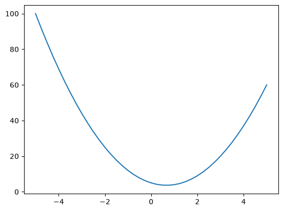

# what is the derivative at a point in the curve?
# df(x)/dx, you used to use the formula nx^(n-1), so our df/dx would be 6x - 4, but we aren't going to do it this way
# we wouldn't write out the expression for neural nets, it would be massive, and 10s of thousands of terms
# we won't take symbolic approach
# instead we use this: lim h->0 (f(x+h)-f(x))/h, the definition asks to take h tends to 0, i.e. very very small value of h, eg. 0.001

#taking h way too small at some point gives incorrect answer cuz we are using floating point arithmetic
# and the representation of all these numbers in computer memory is finite

h = 0.000001
x = 3.0
print("f(3): ", f(x))
print("f(3+h): ", f(x+h))
# slope = derivative = rise/run = change in y / change in x
print("Slope or df/dx at x = 3 using formula: ", (f(x+h) - f(x))/h)
print("f'(x) = 6x-4 = 6*3-4 = 18-4 = 14")

f(3):  20.0
f(3+h):  20.000014000003002
Slope or df/dx at x = 3 using formula:  14.000003002223593
f'(x) = 6x-4 = 6*3-4 = 18-4 = 14

# how about slope at -3
# expectation: if we move at slightly positive direction of x from -3, the function (you can see above) goes down
# so for slope at x+h, we get the slope lower than the slope at -3

h = 0.000001
x = -3.0
print("f(-3): ", f(x))
print("f(-3+h): ", f(x+h))
# slope = derivative = rise/run = change in y / change in x
print("Slope or df/dx at x = 3 using formula: ", (f(x+h) - f(x))/h)
print("f'(x) = 6x-4 = 6*(-3)-4 = -18-4 = -22")

f(-3):  44.0
f(-3+h):  43.999978000003
Slope or df/dx at x = 3 using formula:  -21.999997002808414
f'(x) = 6x-4 = 6*(-3)-4 = -18-4 = -22

# f'(x) = 6x - 4. To find where slope = 0, solve for x, x = 2/3
h = 0.000001
x = 2/3
(f(x+h)-f(x))/h

2.999378523327323e-06

Let’s get a little complex now

# we have 3 inputs, and one output d
# we look at dd/da, dd/db, dd/dc, i.e. derivative of d w.r.t a, b and c

h = 0.0001

# inputs
a = 2.0
b = -3.0
c = 10.0

# to compute dd/da
d1 = a * b + c
a += h # a = 2.0001
d2 = a * b + c
# here, think whether d2 is greater or less than d1
# you might think, oh, a+h>a, so f(x+h)>f(x), wrong!
# if you look at that function carefully, you will see that b is negative, so increasing a causes overall d2 to decrease thus d2<d1
# this will give us the sign of the derivative

print('d1', d1)
print('d2', d2)
print('slope', (d2-d1)/h)
print('verifying slope: dd/da = d(ab + c)/da = b*da/da + dc/da = b*1 + 0 = b =', b)

d1 4.0
d2 3.999699999999999
slope -3.000000000010772
verifying slope: dd/da = d(ab + c)/da = b*da/da + dc/da = b*1 + 0 = b = -3.0

# inputs
a = 2.0
b = -3.0
c = 10.0

# to compute dd/db
d1 = a * b + c
b += h # now testing increase in b.
d2 = a * b + c

print('d1', d1)
print('d2', d2)
print('slope', (d2-d1)/h)
print('verifying slope: dd/db = d(ab + c)/db = a*db/db + dc/db = a*1 + 0 = a =', a)

d1 4.0
d2 4.0002
slope 2.0000000000042206
verifying slope: dd/db = d(ab + c)/db = a*db/db + dc/db = a*1 + 0 = a = 2.0

# similarly for dd/dc too, the result will be 1, it means the rate at which y will increase w.r.t x
# inputs
a = 2.0
b = -3.0
c = 10.0

# to compute dd/dc
d1 = a * b + c
c += h # now testing increase in c.
d2 = a * b + c

print('d1', d1)
print('d2', d2)
print('slope', (d2-d1)/h)
print('verifying slope: dd/dc = d(ab + c)/dc = d(ab)/dc + dc/dc = 0 + 1 = 1')
# this is basically that x=y line, visualize it, with 45 degree angle in that 2d graph of xy plane

d1 4.0
d2 4.0001
slope 0.9999999999976694
verifying slope: dd/dc = d(ab + c)/dc = d(ab)/dc + dc/dc = 0 + 1 = 1

Building Value and drawing the graph¶

# as we know, neural networks will be pretty large expressions, so we need data structures that can maintain these expressions
# starting the core Value object of micrograd and its visualization

# note:
# inside a python class, when a method is declared with name: __something__, they are not just naming conventions, they are functional predefined hooks
# when we use normal syntax, eg. print(a), it internally translates it into method call a.__repr__(), or a.__str__()
# other eg. a + b calls a.__add__(b), len(a) calls a.__len__()
# these are special methods and they are commonly called as:
# DUNDER METHODS
# Python looks for these exact names and calls them automatically
# If Python syntax works on an object, there’s probably a __method__ behind it.
# some common dunder methods:
# def __init__(self):  
#     # runs when object is created (constructor)

# def __repr__(self):  
#     # defines how object is shown in console (debug view)

# def __str__(self):  
#     # defines user-friendly print output

# def __add__(self, other):  
#     # defines behavior of + operator

# def __sub__(self, other):  
#     # defines behavior of - operator

# def __mul__(self, other):  
#     # defines behavior of * operator

# def __truediv__(self, other):  
#     # defines behavior of / operator

# def __len__(self):  
#     # defines behavior of len(obj)

# def __getitem__(self, key):  
#     # defines obj[key] access

# def __setitem__(self, key, value):  
#     # defines obj[key] = value

# def __eq__(self, other):  
#     # defines == comparison

# def __lt__(self, other):  
#     # defines < comparison

# def __call__(self):  
#     # allows object to be called like a function

# def __enter__(self):  
#     # start of 'with' context manager

# def __exit__(self, exc_type, exc, tb):  
#     # end of 'with' block (cleanup)

class Value:
    # constructor, i.e. __init__ runs when object is created, self refers to current instance
    # data is input passed while creating the object
    # the self keyword is not needed for 3 cases a. static method b. class method c. function outside of a class
    # when i call a=Value(1.0), python actually calls Value.__init__(a, 1.0). Thus, we need self.
    # self is not a reserved keyword, you can use any other name and it will function the same as self does. its just a naming convention.
    def __init__(self, data):
        self.data = data

    # __repr__ controls what gets displayed when the object is displayed, without this something ugly cryptic stuff is displayed
    # eg. <__main__.Value object at 0x0000016FC52206E0>
    def __repr__(self):
        return f"Value (data={self.data})"

    def __add__(self, other):
        out = self.data + other.data;#will return scalar, but we want to return a value object
        return Value(out)

    def __mul__(self, other):
        out = self.data * other.data;#will return scalar, but we want to return a value object
        return Value(out)

a = Value(2.0)
b = Value(-3.0)
c = Value(10.0)
print(a.data)
print(a)#calls the __repr__ method when object is displayed at default

# by default, we can't add objects, we can define what should happen by using __add__
print(a+b)
# equivalent to a.__add__(b)

print(a*b + c)
# equivalent to (a.__mul__(b)).__add__(c)

2.0
Value (data=2.0)
Value (data=-1.0)
Value (data=4.0)

Now, we want to introduce multiple other variables/pointers to store intermediate values

class Value:

    # no previous/ node for initial node, eg. input node a, b, c
    def __init__(self, data, _children=()):
        self.data = data
        self._prev = set(_children)

    def __repr__(self):
        return f"Value (data={self.data})"

    # after operation, we also feed in the children of these value objects through self and other
    def __add__(self, other):
        out = self.data + other.data;
        return Value(out, (self, other))

    def __mul__(self, other):
        out = self.data * other.data;
        return Value(out, (self, other))

a = Value(2.0)
b = Value(-3.0)
c = Value(10.0)
d = a * b + c
d

Value (data=4.0)

d._prev

{Value (data=-6.0), Value (data=10.0)}

# so now we know what the actual values of the children were, but not what operation created these values

class Value:

    # no previous/ node for initial node, eg. input node a, b, c
    def __init__(self, data, _children=(), _op='', label=''):
        self.data = data
        self.grad = 0.0 # means no effect initially
        self._prev = set(_children)
        self._op = _op
        self.label = label

    def __repr__(self):
        return f"Value (data={self.data})"

    # after operation, we also feed in the children of these value objects through self and other
    def __add__(self, other):
        out = self.data + other.data;
        return Value(out, (self, other), '+')

    def __mul__(self, other):
        out = self.data * other.data;
        return Value(out, (self, other), '*')

    def tanh(self):
        x = self.data
        t = (math.exp(2*x) - 1)/(math.exp(2*x) + 1)
        out = Value(t, (self, ), 'tanh')
        return out

a = Value(2.0, label='a')
b = Value(-3.0, label='b')
c = Value(10.0, label='c')
e = a*b; e.label='e'
d = e + c
d.label = 'd'
f = Value(-2.0, label='f')
L = d * f; L.label = 'L'

print(d)
print(d._prev)
print(d._op)
print(e)
print(e._prev)
print(e._op)
print(L)

Value (data=4.0)
{Value (data=-6.0), Value (data=10.0)}
+
Value (data=-6.0)
{Value (data=2.0), Value (data=-3.0)}
*
Value (data=-8.0)

# so finally, we know how we are getting the new values(by + or *) and from which values we are getting them
# since the expressions will be larger, we want a way to properly visualize these expressions

Digraph: Directed graph, i.e. every edge has an arrow¶

for undirected graph, use just Graph instead of Digraph¶

Official Documentation:¶

https://graphviz.readthedocs.io/en/stable/
https://graphviz.readthedocs.io/en/stable/api.html

Constructor for digraph:

Digraph(
    name='G',#graph's internal name, usually we don't care about this
    comment=None, #comment for the generated dot file. used for debugging
    filename=None, #when we save the graph, this is written to the file, eg. filename="graph.gv"
    directory=None, #save the graph into images/graph.gv when directory="images"
    format='pdf', #png, pdf, svg(vector graphics, scalable, looks crisp in notebooks), jpg, gif, ps
    engine='dot', #there are different layout algorithms like neato, fdb, circo, twopi. for trees and computation graphs, dot is usually best, and dot is the default one
    encoding='utf-8',
    graph_attr=None, #by default it is Top-Down, i.e. vertical, we can set it to Left-Right using graph_attr={'rankdir':'LR'}
                graph_attr={
                "rankdir":"TB",
                "bgcolor":"black",
                "label":"My Graph"
            }
    node_attr=None,#default style for every node
                node_attr={
                    "shape":"circle",
                    "color":"blue"
                }
    edge_attr=None, #default styling for all edges
                edge_attr={
                    "color":"red"
                }
)

# create a node
# dot.node(
#     name="A",#every node must have a unique name
#     label="Hello"
# )
# uid = str(id(n))
# No two Value objects will have the same id.
# Python guarantees every object has a unique identity during its lifetime. eg. 139832178284912
# label shows what to display
# shape can be "circle" or "record"(box-like sections)
# why record? to include multiple pieces of information (e.g., value and gradient), 
# so a record lets you display them cleanly in compartments.
# dot.edge("A","B") simply means, start directed edge from A and end to B. A ---> B
# dot.edge(uid + n._op, uid). The operation node points to the value node
# id(obj) returns an integer that's unique for that object during its lifetime. 
# then convert it to string cuz graphviz expects node names as strings
# { data 3.1416 }

# a = Value(2)
# b = Value(3)
# c = a + b

# internally
# a._op = ""
# b._op = ""
# c._op = "+"
c._prev = {a, b}

# trace(c) will produce
# nodes = {a, b, c}
# edges = {
#     (a, c),
#     (b, c)
# }

# suppose:
# id(a) = 101
# id(b) = 102
# id(c) = 103

# then we create nodes during node creation process as:
# dot.node("101", ...)      # a
# dot.node("102", ...)      # b
# dot.node("103", ...)      # c
# dot.node("103+", label="+")   # operation node +: created during: dot.node(name=uid + n._op, label=n._op)

# so for this part of edge creation:
# for n1, n2 in edges:
    # dot.edge(str(id(n1)), str(id(n2)) + n2._op)
# dot.edge("101", "103+")
# draws arrows within existing nodes

# Note:
# The child (n1) is represented by its value node (id(n1)).
# The parent/result (n2) is represented by two nodes:
    # an operation node (id(n2) + n2._op), and
    # a value node (id(n2)).
# The graph connects:
    # child value → operation, then
    # operation → result value.

# the operator nodes are not a part of the graph, and they are drawn only during display, i.e. during draw_dot() method

from graphviz import Digraph

def trace(root):
    # builds a set of all nodes and edges in a graph
    nodes, edges = set(), set()
    def build(v):
        if v not in nodes:
            nodes.add(v)
            for child in v._prev:
                edges.add((child, v))
                build(child)
    build(root)
    return nodes, edges

def draw_dot(root):
    dot = Digraph(format='svg', graph_attr={'rankdir':'LR'}) #LR = left to right

    nodes,edges = trace(root)

    # create nodes
    for n in nodes:
        uid = str(id(n))#need a unique identifier for each node in the graph

        # for any value in the graph, create a rectangular ('record') node for it
        dot.node(name = uid, label = f"{{ {n.label:s} | data {n.data:.4f} | grad {n.grad:.4f}}}", shape='record')
        if n._op:
            # if this value is a result of some operation, create an operator node for it
            # we need unique name for operator node too, internally it's name uses name of output node
            # but in label, just display it as + or *
            dot.node(name = uid + n._op, label = n._op)

            # then connect this operator node with our value node
            # i understand it now, wow
            dot.edge(uid + n._op, uid)

    # create connections
    for n1, n2 in edges:
        # connect n1 to the op node of n2
        # draw an arrow from existing node id(n1) to id(n2)+op(if op doesnt exist, it is empty anyway)
        dot.edge(str(id(n1)), str(id(n2)) + n2._op)

    return dot

draw_dot(L)

Manual backpropagation¶

# we are able to do this forward pass. The output of this forward pass is -8
# now we want to do backpropagation, we start at L, then we go backwards and calculate the gradient along all these intermediate values
# i.e. for each of these intermediate nodes, we are computing their derivative w.r.t L
# dL/dL = 1
# some of these parameters will be weights, and then we can know how the weights impact the loss function
# dOutput/dLeafnodes, leaf nodes: data itself, weights
# we don't want or use dL/dInputNode as the value of input data is fixed
# but the weights will be iteratively adjusted using gradient information
# we want a variable inside the value class that will store the derivative of L w.r.t that value, and we will call this grad
# initially set the grad value to 0, i.e. no effect of input on output, i.e. change in this input doesn't change output
# eg. f.grad = dL/df
# now we fill in these gradients and do backpropagation manually

# start from the parent node
# dL/dL: when L is changed by h, how much is L changed by? answer: also h, so 1

def lol():

    h = 0.001
    
    a = Value(2.0, label='a')
    b = Value(-3.0, label='b')
    c = Value(10.0, label='c')
    e = a*b; e.label='e'
    d = e + c
    d.label = 'd'
    f = Value(-2.0, label='f')
    L = d * f; L.label = 'L'
    L1 = L.data

    a = Value(2.0, label='a')
    b = Value(-3.0, label='b')
    c = Value(10.0, label='c')
    # c.data += h
    e = a*b; e.label='e'
    e.data += h
    d = e + c
    # d.data += h
    d.label = 'd'
    f = Value(-2.0, label='f')
    L = d * f; L.label = 'L'
    L2 = L.data

    print((L2 - L1)/h)

#to find: dL/da, do a = Value(2.0 + h, label='a')
# to find: dL/dL, do L2 = L.data + h
# to find: dL/df, do f = Value(-2.0 + h, label='f')
# to find: dL/dd, do d.data += h
lol()

-2.000000000000668

# so in our manual backpropagation, we directly set L.grad = 1.0
L.grad = 1.0
draw_dot(L)

# now we do dL/dd and dL/df
L = d * f
dL/dd = ?. Ans: f
proof:
(f(x+h)-f(x))/h, f(x) = L
= ((d+h)*f - d*f)/h
= (df + hf - df)/h
= (hf)/h
= f
Symmetrically, dL/df = d

So, d.grad = Value(f)
and, f.grad = Value(d)

print(d.data)
print(f.data)
f.grad = d.data
d.grad = f.data
draw_dot(L)

4.0
-2.0

# now to derive dL/dc
# this is the crux of backpropagation
# we know impact of d on L, and impact of c on d, and impact of e on d, but how to find how c impacts L? dL/dc?
# chain rule
# if a car travels twice as fast as a bicycle, and the bicycle is 4x as fast as a man
# then the car travels 2*4=8 times as fast as the man

dd/dc = ?
dd/de = ?
d = c + e
dd/dc = 1.0

(f(x+h) - f(x))/h
= ((c+h+e)-(c+e))/h
= (c+h+e-c-e)/h
= h/h
= 1

By symmetry, dd/de = 1.0
# this is local derivative, cuz we are concerned only on influence of c on d and e on d

dL/dc = ?
we have, dL/dd, dd/dc
So, dL/dc = (dL/dd) * (dd/dc)
dL/dc = (dL/dd) * 1
# So a plus node just routes the gradient
Similarly, dL/de = (dL/dd) * (dd/de) = (dL/dd) * 1
dL/dd = -2.0
dL/de = -2.0

c.grad = d.grad;
e.grad = d.grad;

draw_dot(L)

# now we find a.grad and b.grad, i.e. dL/da and dL/db
dL/da = (dL/de)*(de/da)
dL/db = (dL/de)*(de/db)

So, de/da = d(a*b)/da = b and 
    de/db = a
Earlier we found that criss cross type of relationship, we are going to reuse that concept
We already know, dL/de = e.grad
so, dL/da = (e.grad) * b.data
    dL/db = (e.grad) * a.data

print(a.data)
print(b.data)
print(e.grad)

a.grad = e.grad * b.data
b.grad = e.grad * a.data
draw_dot(L)

2.0
-3.0
-2.0

# verify again
# start from the parent node
# dL/dL: when L is changed by h, how much is L changed by? answer: also h, so 1

def lol():

    h = 0.001
    
    a = Value(2.0, label='a')
    b = Value(-3.0, label='b')
    c = Value(10.0, label='c')
    e = a*b; e.label='e'
    d = e + c
    d.label = 'd'
    f = Value(-2.0, label='f')
    L = d * f; L.label = 'L'
    L1 = L.data

    a = Value(2.0, label='a')
    # a.data += h
    b = Value(-3.0, label='b')
    b.data += h
    c = Value(10.0, label='c')
    # c.data += h
    e = a*b; e.label='e'
    # e.data += h
    d = e + c
    # d.data += h
    d.label = 'd'
    f = Value(-2.0, label='f')
    L = d * f; L.label = 'L'
    L2 = L.data

    print((L2 - L1)/h)

lol()

-3.9999999999995595

# so, we iterated through all the nodes one by one and locally applied the chain rule to find the gradient
# for any node, we can always find its gradient, i.e. dL/dN
# so backpropagation is just recursive application of chain rule backwards through the computational graph
# so now lets see this power in action briefly
# we are going to make the value of nudge our inputs so that our L goes up
# so for L to move up, we move a.data in the direction of the gradient, i.e. a.data += a.grad
# so the code below is just one step of optimization that we are running
# these gradients give us some power to influence the final output, and this is really useful for training knowledge

print('Before:', L.data)

a.data += 0.01 * a.grad #step_size = 0.01
b.data += 0.01 * b.grad
c.data += 0.01 * c.grad
f.data += 0.01 * f.grad
# these are the leaf nodes that we have control over
# NOTE: if we nudge in the direction of the gradient, we expect L to go up positively, so if it is -8, it should go to -6 or something

# rewriting the forward pass
e = a * b
d = e + c
L = d * f

print('After:', L.data)

Before: -8.0
After: -7.286496

Backpropagating through a neuron¶

One more example of manual backpropagation but with complex and useful example¶

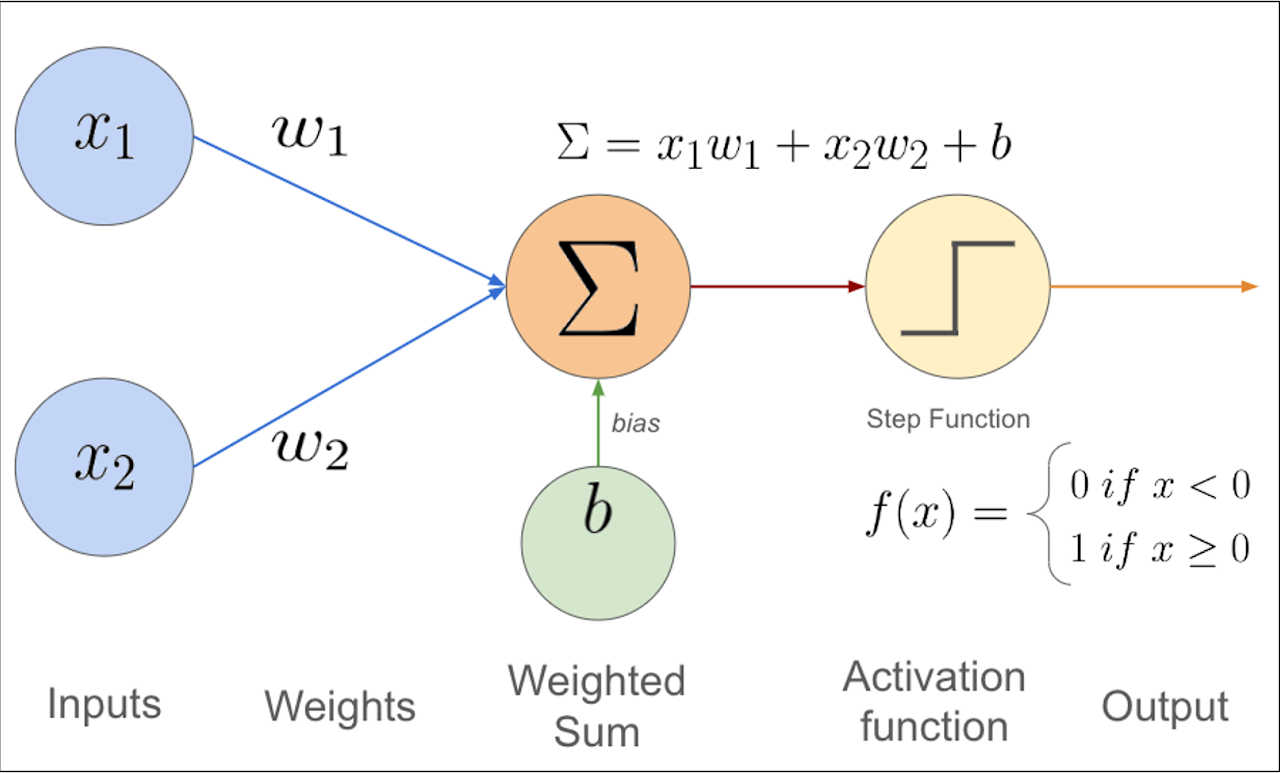
# we're going to backpropagate through a neuron
# bias: sort of innate trigger happiness of a neuron, something that is specific to a neuron and independent of the input
# activation function: sigmoid or tanh, sort of a squishing function

plt.plot(np.arange(-5, 5, 0.2), np.tanh(np.arange(-5, 5, 0.2)))
plt.grid()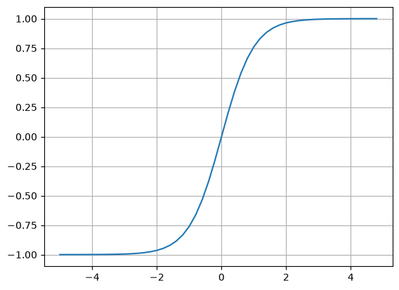

# numpy has np.tanh
# the inputs get squashed on the y coordinate
# the function will only go upto 1, we cap it smoothly at 1 and -1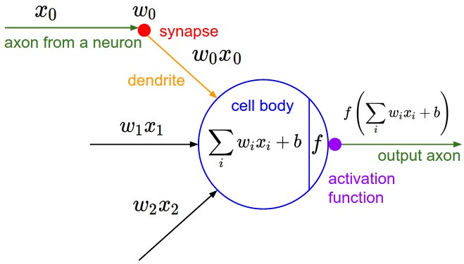

Open original image: neuron_model.jpeg

Open original image: twoinputnn.png

Open original image: tanh.svg

# inputs x1, x2
x1 = Value(2.0, label='x1')
x2 = Value(0.0, label='x2')

# weights w1, w2
w1 = Value(-3.0, label='w1')
w2 = Value(1.0, label='w2')

# bias of the neuron
# for just education purposes, we want to see nice output values so setting this value explicitly
# in real projects, it doesn't matter
b = Value(6.8813735870195432, label='b')

# x1w1 + x2w2 + b
x1w1 = x1 * w1
x1w1.label = 'x1w1'
x2w2 = x2 * w2
x2w2.label = 'x2w2'

x1w1x2w2 = x1w1 + x2w2
x1w1x2w2.label = 'x1w1 + x2w2'

n = x1w1x2w2 + b
n.label = 'n'

# tanh is a hyperbolic function
o = n.tanh()#we added the tanh method at this point of time
o.label = 'o'

draw_dot(o)

# now we do backpropagation and fill up all the gradients
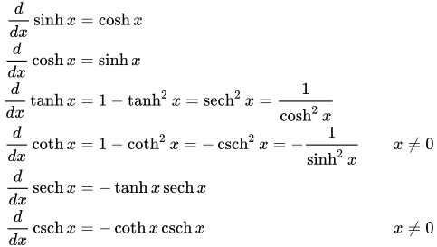
o.grad = 1.0

draw_dot(o)

# to backpropagate through tanh, we need to know the local derivative of tanh
# o = tanh(n)
# do/dn = n.grad = ?
# we could do our derivative in above formula as: d(e^(2n-1)/e^(2n+1))/dn
# do/dn = 1 - o**2
print(1 - o.data**2)
n.grad = 1 - o.data ** 2

0.4999999999999999

Open original image: dtanh.svg

draw_dot(o)

# now to find gradient w.r.t x1w1+x2w2 and b
# from our previous knowledge, we know that, in case of addition, gradient is just going to flow/route through normally
x1w1x2w2.grad = n.grad
b.grad = n.grad

draw_dot(o)

# similar for x1w1 and x2w2
x1w1.grad = x1w1x2w2.grad
x2w2.grad = x1w1x2w2.grad

draw_dot(o)

# from our earlier example, we have detected a pattern in multiplication case too
x2.grad = w2.data * x2w2.grad
w2.grad = x2.data * x2w2.grad

# note that since x2 is 0, we see that w2.grad = 0
# this is because, since x2 is 0, no matter how we change w2, it has no effect on the final output

x1.grad = w1.data * x1w1.grad
w1.grad = x1.data * x1w1.grad

draw_dot(o)

Automating the backward pass¶

# so if we want the neurons output to increase, we move in the direction of the gradient
# obviously we won't implement backpropagation manually, so now we automate backpropagation for each operation

# create cell notes later as to why some variables start with _ and why some don't
class Value:

    def __init__(self, data, _children=(), _op='', label=''):
        self.data = data
        self.grad = 0.0

        # this will be a function which will implement our chain rule at each node
        # by default: it will be a function that doesn't do anything, i.e. empty function, and this is the case for a leaf node
        # as we have seen, this differs for addition and multiplication
        self._backward = lambda: None
        self._prev = set(_children)
        self._op = _op
        self.label = label

    def __repr__(self):
        return f"Value (data={self.data})"

    # after operation, we also feed in the children of these value objects through self and other
    def __add__(self, other):
        out = Value(self.data + other.data, (self, other), '+');

        def _backward():
            # our job is to take out.grad then somehow propagate it into self.grad and other.grad
            # for addition it was simple, it just flows as we have seen in 2 previous examples
            self.grad = out.grad
            other.grad = out.grad

        out._backward = _backward
        return out

    def __mul__(self, other):
        out = Value(self.data * other.data, (self, other), '*')

        def _backward():
            self.grad = out.grad * other.data
            other.grad = out.grad * self.data

        out._backward = _backward
        return out

    def tanh(self):
        x = self.data
        t = (math.exp(2*x) - 1)/(math.exp(2*x) + 1)
        out = Value(t, (self, ), 'tanh')

        def _backward():
            self.grad = (1 - t**2)*out.grad
            
        out._backward = _backward
        return out

# repeat the same process as earlier, but we don't do it manually anymore
# inputs x1, x2
x1 = Value(2.0, label='x1')
x2 = Value(0.0, label='x2')

# weights w1, w2
w1 = Value(-3.0, label='w1')
w2 = Value(1.0, label='w2')

# bias of the neuron
# for just education purposes, we want to see nice output values so setting this value explicitly
# in real projects, it doesn't matter
b = Value(6.8813735870195432, label='b')

# x1w1 + x2w2 + b
x1w1 = x1 * w1
x1w1.label = 'x1w1'
x2w2 = x2 * w2
x2w2.label = 'x2w2'

x1w1x2w2 = x1w1 + x2w2
x1w1x2w2.label = 'x1w1 + x2w2'

n = x1w1x2w2 + b
n.label = 'n'

# tanh is a hyperbolic function
o = n.tanh()#we added the tanh method at this point of time
o.label = 'o'

draw_dot(o)

# as a base case, we need to set o.grad to 1, cuz initially it is 0, and multiplying it by 0 results inaccurate answers for all inputs/weights/bias/etc
o.grad = 1
draw_dot(o)

# instead of manually setting each gradient value for an input, weight or etc, we automate it
# we call ._backward() in right order
o._backward()
draw_dot(o)

n._backward()
draw_dot(o)

# we can call it on a leaf node, but nothing will happen
b._backward()
draw_dot(o)

x1w1x2w2._backward()
draw_dot(o)

x1w1._backward()
draw_dot(o)

x2w2._backward()
draw_dot(o)

# so one last piece, we are calling _backward manually many times, we want to ensure doing it only once is enough
# first we need to ensure that everything is already in place before doing backpropagation
# everything needed should be there
# this ordering of graphs can be achieved using topological sort: it is the laying out of a graph such that all edges go only from left to right

# Purpose of topological sort:
# Figure out the correct order to perform backpropagation.
# Key rule: A node can only be processed after all the nodes that depend on it have been processed.

# remember:
# c = a * b
# c._prev = {a, b}

# trace an example for topological sort:
# a = Value(2)
# b = Value(3)
# c = a * b
# d = c + a

# build_topo(d)
        # status:
        # topo = []#remembers the order, provides the order to backprop, thus maintained in a list as it preserves order of append
        # visited = {}#remembers whether we have seen the node or not, so it is a set: fast to check membership, no need to worry about order
# we're at d, d is not visited so add d, visited = {d}
# parents of d are c and a
# visit c
# visited = {d, c}
# parents of c are a and b
# visit a
# visited = {d, c, a}
# parents of a: None, so append it to topo as well
# topo = [a] return
# build_topo(b) is called as previously for other nodes d, c and a
# visited = {d,c,a,b}
# parents of b: None, so append it to topo as well
# topo = [a, b]
# we back at c now, append it to topo too
# topo = [a, b, c]
# topo = [a, b, c, d]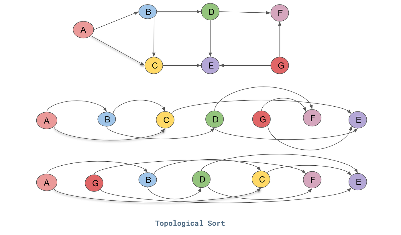

Open original image: topologicalsort.png

# implementing topological sort
# simply ensure that you're in a list only after all the children required to process you are already in the list, this list is provided by topo
topo = []
visited = set()

def build_topo(v):
    if v not in visited:
        visited.add(v)# Don't visit this node twice.

        # Visit all of this node's parents first.
        for child in v._prev:
            build_topo(child)

        # After all parents are processed, add this node
        topo.append(v)

build_topo(o)
topo

[Value (data=6.881373587019543),
 Value (data=-3.0),
 Value (data=2.0),
 Value (data=-6.0),
 Value (data=0.0),
 Value (data=1.0),
 Value (data=0.0),
 Value (data=-6.0),
 Value (data=0.8813735870195432),
 Value (data=0.7071067811865476)]

# let's reset the gradients
# repeat the same process as earlier, but we don't do it manually anymore
# inputs x1, x2
x1 = Value(2.0, label='x1')
x2 = Value(0.0, label='x2')

# weights w1, w2
w1 = Value(-3.0, label='w1')
w2 = Value(1.0, label='w2')

# bias of the neuron
# for just education purposes, we want to see nice output values so setting this value explicitly
# in real projects, it doesn't matter
b = Value(6.8813735870195432, label='b')

# x1w1 + x2w2 + b
x1w1 = x1 * w1
x1w1.label = 'x1w1'
x2w2 = x2 * w2
x2w2.label = 'x2w2'

x1w1x2w2 = x1w1 + x2w2
x1w1x2w2.label = 'x1w1 + x2w2'

n = x1w1x2w2 + b
n.label = 'n'

# tanh is a hyperbolic function
o = n.tanh()#we added the tanh method at this point of time
o.label = 'o'

draw_dot(o)

o.grad = 1.0

topo = []
visited = set()
def build_topo(v):
    if v not in visited:
        visited.add(v)
        for child in v._prev:
            build_topo(child)
        topo.append(v)
build_topo(o)

# ensure that we start backpropagation from parent and ending upto leaf nodes
for node in reversed(topo):
    node._backward()

draw_dot(o)

MAIN BACKPROPAGATION CODE¶

# now we want to hide this functionality inside the Value class
# create cell notes later as to why some variables start with _ and why some don't
class Value:

    def __init__(self, data, _children=(), _op='', label=''):
        self.data = data
        self.grad = 0.0

        # this will be a function which will implement our chain rule at each node
        # by default: it will be a function that doesn't do anything, i.e. empty function, and this is the case for a leaf node
        # as we have seen, this differs for addition and multiplication
        self._backward = lambda: None
        self._prev = set(_children)
        self._op = _op
        self.label = label

    def __repr__(self):
        return f"Value (data={self.data})"

    # after operation, we also feed in the children of these value objects through self and other
    def __add__(self, other):
        out = Value(self.data + other.data, (self, other), '+');

        def _backward():
            # our job is to take out.grad then somehow propagate it into self.grad and other.grad
            # for addition it was simple, it just flows as we have seen in 2 previous examples
            self.grad += out.grad
            other.grad += out.grad

        out._backward = _backward
        return out

    def __mul__(self, other):
        out = Value(self.data * other.data, (self, other), '*')

        def _backward():
            self.grad += out.grad * other.data
            other.grad += out.grad * self.data

        out._backward = _backward
        return out

    def tanh(self):
        x = self.data
        t = (math.exp(2*x) - 1)/(math.exp(2*x) + 1)
        out = Value(t, (self, ), 'tanh')

        def _backward():
            self.grad += (1 - t**2)*out.grad
            
        out._backward = _backward
        return out

    # define an actual backward propagation function that does everything
    def backward(self):
        topo = []
        visited = set()
        def build_topo(v):
            if v not in visited:
                visited.add(v)
                for child in v._prev:
                    build_topo(child)
                topo.append(v)
        build_topo(self)
        
        self.grad=1.0
        for node in reversed(topo):
            node._backward()

# let's reset the gradients
# repeat the same process as earlier, but we don't do it manually anymore
# inputs x1, x2
x1 = Value(2.0, label='x1')
x2 = Value(0.0, label='x2')

# weights w1, w2
w1 = Value(-3.0, label='w1')
w2 = Value(1.0, label='w2')

# bias of the neuron
# for just education purposes, we want to see nice output values so setting this value explicitly
# in real projects, it doesn't matter
b = Value(6.8813735870195432, label='b')

# x1w1 + x2w2 + b
x1w1 = x1 * w1
x1w1.label = 'x1w1'
x2w2 = x2 * w2
x2w2.label = 'x2w2'

x1w1x2w2 = x1w1 + x2w2
x1w1x2w2.label = 'x1w1 + x2w2'

n = x1w1x2w2 + b
n.label = 'n'

# tanh is a hyperbolic function
o = n.tanh()#we added the tanh method at this point of time
o.label = 'o'

draw_dot(o)

o.backward()

draw_dot(o)

Shared nodes and gradient accumulation¶

ONE BUG FIX¶

# we have one bug to fix
# when one node is used multiple times

# simplest case that shows the bug
a = Value(3.0, label='a')
b = a + a; b.label = 'b';
b.backward()
draw_dot(b)
# there are actually 2 arrows on top of one another
# the gradient is not correct as db/da = 2

# this cell runs the same code but after fixing the bug above

a = Value(3.0, label='a')
b = a + a; b.label = 'b';
b.backward()
draw_dot(b)
# there are actually 2 arrows on top of one another
# the gradient is now correct as db/da = 2

a = Value(-2.0, label='a')
b = Value(3.0, label='b')
d = a * b; d.label='d'
e = a + b; e.label = 'e'
f = d * e; f.label = 'f'

f.backward()
draw_dot(f)

# run same code as in above cell but after fixing the bug

a = Value(-2.0, label='a')
b = Value(3.0, label='b')
d = a * b; d.label='d'
e = a + b; e.label = 'e'
f = d * e; f.label = 'f'

f.backward()
draw_dot(f)

# the bug occurs when a variable gets used more than once
# in above eg. when we are backpropagating, and we are at e, then we write a value to a and b 's gradient
# then after processing e, when we process d, we simply overwrite to a and b's gradient
# look at multivariate case of chain rule and its generalization 
# the solution is to accumulate/add these gradients
# so in the Value class, we just use += instead of just =
# bug fix was very simple, for all three _backward methods, use +=
# eg for one of the cases:
        # def _backward():
        #     self.grad += out.grad * other.data
        #     other.grad += out.grad * self.data

Extending the engine¶

minor additions, add exponential, division, rmul, sub etc features¶

# now we want to hide this functionality inside the Value class
# create cell notes later as to why some variables start with _ and why some don't
class Value:

    def __init__(self, data, _children=(), _op='', label=''):
        self.data = data
        self.grad = 0.0

        # this will be a function which will implement our chain rule at each node
        # by default: it will be a function that doesn't do anything, i.e. empty function, and this is the case for a leaf node
        # as we have seen, this differs for addition and multiplication
        self._backward = lambda: None
        self._prev = set(_children)
        self._op = _op
        self.label = label

    def __repr__(self):
        return f"Value (data={self.data})"

    # after operation, we also feed in the children of these value objects through self and other
    def __add__(self, other):
        other = other if isinstance(other, Value) else Value(other)
        out = Value(self.data + other.data, (self, other), '+');

        def _backward():
            # our job is to take out.grad then somehow propagate it into self.grad and other.grad
            # for addition it was simple, it just flows as we have seen in 2 previous examples
            self.grad += out.grad
            other.grad += out.grad

        out._backward = _backward
        return out

    def __radd__(self, other):
        return self + other
    
    def __mul__(self, other):
        other = other if isinstance(other, Value) else Value(other)
        out = Value(self.data * other.data, (self, other), '*')

        def _backward():
            self.grad += out.grad * other.data
            other.grad += out.grad * self.data

        out._backward = _backward
        return out

    def __rmul__(self, other): #other*self
        return self * other

    def __neg__(self): #-self
        return self * -1

    def __sub__(self, other): # self - other
        return self + (-other)

    def __rsub__(self, other): # self - other
        return other + (-self)#__radd__ already knows how to convert other to a value

    def __pow__(self, other):
        assert isinstance(other, (int, float)), "only supporting int/float powers for now"
        out = Value(self.data**other, (self, ), f'**{other}')

        # d(x^n)/dx = nx^(n-1), assuming n is a constant
        def _backward():
            # good job figuring this out yourself!
            self.grad += out.grad * (other * (self.data**(other - 1)))

        out._backward = _backward
        return out

    def __truediv__(self, other): #self/other
        return self * other**-1

    def tanh(self):
        x = self.data
        t = (math.exp(2*x) - 1)/(math.exp(2*x) + 1)
        out = Value(t, (self, ), 'tanh')

        def _backward():
            self.grad += (1 - t**2)*out.grad
            
        out._backward = _backward
        return out

    def exp(self):
        x = self.data
        out = Value(math.exp(x), (self, ), 'exp')

        # we know that de^x/dx = e^x: good job, but we missed that out.data part
        def _backward():
            self.grad += out.data * out.grad

        out._backward = _backward
        return out
        
    # define an actual backward propagation function that does everything
    def backward(self):
        topo = []
        visited = set()
        def build_topo(v):
            if v not in visited:
                visited.add(v)
                for child in v._prev:
                    build_topo(child)
                topo.append(v)
        build_topo(self)
        
        self.grad=1.0
        for node in reversed(topo):
            node._backward()

# inputs x1, x2
x1 = Value(2.0, label='x1')
x2 = Value(0.0, label='x2')

# weights w1, w2
w1 = Value(-3.0, label='w1')
w2 = Value(1.0, label='w2')

# bias of the neuron
# for just education purposes, we want to see nice output values so setting this value explicitly
# in real projects, it doesn't matter
b = Value(6.8813735870195432, label='b')

# x1w1 + x2w2 + b
x1w1 = x1 * w1
x1w1.label = 'x1w1'
x2w2 = x2 * w2
x2w2.label = 'x2w2'

x1w1x2w2 = x1w1 + x2w2
x1w1x2w2.label = 'x1w1 + x2w2'

n = x1w1x2w2 + b
n.label = 'n'

# tanh is a hyperbolic function
o = n.tanh()#we added the tanh method at this point of time
o.label = 'o'

o.backward()
draw_dot(o)

# first we want to conveniently do something like Value(2.0) + 1, kind of like operator overloading but by cheating
# in our code, we assume that if the element after the + sign is not a Value object, then it is an integer, so convert it into value object then add
# other = other if isinstance(other, Value) else Value(other)
a = Value(2.0)
print(a+1)
print(a*3)
print(2*a)
print(a.exp())

Value (data=3.0)
Value (data=6.0)
Value (data=4.0)
Value (data=7.38905609893065)

# but its annoying that 2 * a, or 1 + a wont work
# this is because a + 2 calls a.__add__(2) but 2 + a calls 2.__add__(a)
# while we can modify the method of a since it is a Value object that we created
# we can't risky modifying the add method of 2 i guess if it is even possible

# buuut
# there is something called the __rmul__ which acts like a fallback
# so if python can't do 2*a cuz it gives error, it will try doing a * 2 instead

a/b = a * (1/b) = a * (b**-1)¶

so for division we actually want to implement a^b instead of a/b¶

a = Value(2.0)
b = Value(4.0)
print(a/b)
a - b

Value (data=0.5)

Value (data=-2.0)

Let’s focus on what we were working on previously, we break up tanh and exercise with more operations¶

Open original image: tanh.svg

# inputs x1, x2
x1 = Value(2.0, label='x1')
x2 = Value(0.0, label='x2')

# weights w1, w2
w1 = Value(-3.0, label='w1')
w2 = Value(1.0, label='w2')

# bias of the neuron
# for just education purposes, we want to see nice output values so setting this value explicitly
# in real projects, it doesn't matter
b = Value(6.8813735870195432, label='b')

# x1w1 + x2w2 + b
x1w1 = x1 * w1
x1w1.label = 'x1w1'
x2w2 = x2 * w2
x2w2.label = 'x2w2'

x1w1x2w2 = x1w1 + x2w2
x1w1x2w2.label = 'x1w1 + x2w2'

n = x1w1x2w2 + b
n.label = 'n'
# -------
# tanh is a hyperbolic function
# o = n.tanh()
# use the given formula above instead of using tanh directly from Value class
# e^(2x) = (2*n).exp()

e = (2*n).exp()
o = (e-1)/(e+1)

# why do we do this, 
# we want to see different graph, in this case the graph is longer, but the operations are mathematically equivalent
# here we are replacing single tanh with use of exponentiation, division, etc.
# we want to see the same result in o.data as forward pass is the same
# and we also want to see the same result in leaf nodes w1.grad, x1.grad, w2.grad, x2.grad because of mathematical equivalence

# -------

o.label = 'o'
# o.grad= 1.0, no need here cuz already implemented inside the backward() method of Value class
o.backward()
draw_dot(o)

# summary: the level at which you implement the operations is totally upto you, and we got to work with different operators

Comparing with PyTorch¶

NOW WE DO THE EXACT SAME THING, BUT BY USING A MODERN DEEP NEURAL NETWORK LIBRARY: PYTORCH¶

# Notes:
# micrograd is a scalar valued engine, so we only have scalar values like 2.0
# but in pytorch everything is based around tensors, and tensors are just n-dimensional arrays of scalars

import torch
print(torch.Tensor([[1,2,3], [4,5,6]]))
torch.Tensor([[1,2,3], [4,5,6]]).shape

tensor([[1., 2., 3.],
        [4., 5., 6.]])

torch.Size([2, 3])

torch.Tensor([2.0])

tensor([2.])

torch.Tensor([2.0]).double()
# in below code, we cast to double because python is by default using double precision for its floating point numbers
# by default datatype of float tensors is float32 (i.e. single precision float)
# so we cast it to double so that we have float64 just like in python

tensor([2.], dtype=torch.float64)

# by default pytorch assumes that nodes don't require gradients, i.e. set to false for efficiency reasons, cuz no need of gradients for leaf nodes
# thus we need to explictly state that all nodes require gradients

import torch

x1=torch.Tensor([2.0]).double(); x1.requires_grad = True
x2=torch.Tensor([0.0]).double(); x2.requires_grad = True
w1=torch.Tensor([-3.0]).double(); w1.requires_grad = True
w2=torch.Tensor([1.0]).double(); w2.requires_grad = True
b = torch.Tensor([6.8813735870195432]).double(); b.requires_grad=True
n = x1*w1 + x2*w2 + b
o = torch.tanh(n)

print(o.data.item())#.item() takes single tensor of one element and it just returns that element stripping out the tensor
o.backward()

print('---')
print('x2', x2.grad.item())
print('w2', w2.grad.item())
print('x1', x1.grad.item())
print('w1', w1.grad.item())

# cross checked with our implementation, and it works perfectly

0.7071066904050358
---
x2 0.5000001283844369
w2 0.0
x1 -1.5000003851533106
w1 1.0000002567688737

tensor([0.7071], dtype=torch.float64, grad_fn=<TanhBackward0>)

o.data

tensor([0.7071], dtype=torch.float64)

o.item()

0.7071066904050358

# adv of pytorch: it can do what we did with tensors as a special case when our tensors are all single element tensors
# but big deal is that everything is very efficient because we are working with these tensor objects, we can do everything in parallel on all of these tensors

Neurons, layers and the MLP¶

building a neural net library (multi-layer perceptron) in micrograd¶

# since we now have machinery enough to build complicated mathematical expressions
# we can also start building neural nets (neural nets are just a specific class of mathematical expressions)

Original note stored inside an HTML comment

<!---

a neuron stores a bias and multiple weights.
Suppose we have 3 inputs: x = [2.0, 3.0, -1.0]
Suppose we randomly initialize weights and biases as:
w = [0.5, -0.2, 0.8]
b = 0.1
The neuron computes: x1*w1 + x2*w2 + x3*w3 + b = -0.3
Then it applies tanh: tanh(-0.3) is the neuron's output

1. Neuron initialization:
"Create a neuron that expects 3 inputs."
Neuron(3)
class Neuron:
    def __init__(self, nin): #nin: number of inputs
    
self.w = [Value(random.uniform(-1,1)) for _ in range(nin)]
this creates a list of Value objects (not floats)
[
 Value(0.27),
 Value(-0.91),
 Value(0.63)
]
Why Value objects? cuz we want gradients later

self.b = Value(random.uniform(-1,1))
creates a bias, and each neuron has 1 bias

--- forward pass ---
def __call__(self, x):
instead of using a named forward method, karpathy prefers to use n(x) which calls Neuron.__call__(n, x)

--- zip ---
suppose:
weights: [0.5, -0.2, 0.8]
inputs: [2, 3, -1]
then zip(self.w, x) produces:
	(0.5, 2)
	(-0.2, 3)
	(0.8, -1)
its like merging two lists together
then generator produces something like this after multiplication:
		1.0
		-0.6
		-0.8
		
then act = sum((wi*xi for wi,xi in zip(self.w, x)), self.b)
is equivalent to bias + w1x1 + w2x2 + ... + wnxn
then out = tanh(act)

-----That's it for a single neuron, a neuron's process can be summarized as: n inputs -> weighted sum -> tanh -> one output-----

Now, lets talk about a layer
A layer is just many neurons side by side
eg. Layer(3,4) means there are 4 neurons in a layer and each of the four neurons receive 3 inputs x1,x2 and x3 each.
suppose x = [2,3,-1]
neuron 1 computes n1(x)
neuron 2 computes n2(x)
neuron 3 computes n3(x)
neuron 4 computes n4(x)

Layer initialization:
self.neurons = [Neuron(nin) for _ in range(nout)]
Suppose Layer(3,4)
then python builds [Neuron(3),Neuron(3),Neuron(3),Neuron(3)]
and each neuron(3) has 3 weights and one bias

---Layer's forward pass---
outs = [n(x) for n in self.neurons]
This code is equivalent to this:
outs = []
for n in self.neurons:
    outs.append(n(x))

then output is outs=[0.7,-0.3,0.9,0.1]


---- MLP ----
its just a list of layers, nothing more
MLP(3,[4,4,1])
it means, 3 inputs, 1 layer with 4 neurons, 1 layer with 4 neurons, 1 layer with 1 neuron

----
sz = [nin] + nouts
suppose nin = 3 and nouts = [4,4,1]
then sz = [3,4,4,1]
why do we need this?
because every adjacent pair tells us how to build one layer accordingly
as: 3-4, 4-4 and 4-1

---
self.layers = [
    Layer(sz[i], sz[i+1])
    for i in range(len(nouts)): for i in range(3) which matches count
]
This code creates:
Layer(3,4)
Layer(4,4)
Layer(4,1)


------ FORWARD PASS THROUGH MLP ---
Suppose x=[2,3,-1]
First layer: Layer(3,4) returns [0.2,0.5,-0.1,0.8]
cuz first layer has 4 neurons, 1 neuron returns one output
Then x = layer(x)
i.e. x = [0.2,0.5,-0.1,0.8]
Next layer: Layer(4,4) returns [-0.4,0.3,0.9,-0.2]
Now x = [-0.4,0.3,0.9,-0.2]
Final layer Layer(4,1) returns 0.73
So the network's prediction is 0.73

Parameter count for MLP(3, [4, 4, 1])
For hidden layer 1: 3 weights * 4 neurons + 4 biases = 16
For hidden layer 2: 4 weidghts * 4 neurons + 4 biases = 20
For last layer: 1 weight * 4 neurons + 1 bias = 5
Grand total: 41 parameters
Each one of these 41 parameters is a Value object, and after calling backward(), each Value object will have a .grad that tells us how to adjust the parameters during learning.

---!>

import random

class Neuron:
    def __init__(self, nin): #nin: number of inputs to a neuron
        self.w = [Value(random.uniform(-1,1)) for _ in range(nin)] # a weight that is a random num between -1 and 1
        self.b = Value(random.uniform(-1,1)) # a bias that controls the overall trigger happiness of this neuron

    # we want to do the forward pass of the neuron instead
    # first we want to multiply all pairs of w with x: i.e. x1w1 + x2w2 + ... + xnwn
    # zip takes 2 iterators and creates a new iterator that iterates over the tuples of their corresponding entries
    # act = w1x1 + w2x2 + ... + wnxn + b

    # actually, sum takes a second optional parameter which is the start value, and by default it is 0.0, but we can start with self.b making it more efficient
    
    def __call__(self, x):
        # w*x + b
        # act = sum(wi*xi for wi,xi in zip(self.w, x), 0.0) + self.b
        act = sum((wi*xi for wi,xi in zip(self.w, x)), self.b)
        out = act.tanh()# pass the activation through non-linearity
        return out

    def parameters(self):
        return self.w + [self.b] # just return a concatenated list of weights and biases of a neuron. since self.b was single value object and not a list

# a layer is literally just a list of neurons
class Layer:

    # 2 args: input: how many neurons we have, output: how many neurons do we want in our layer
    def __init__(self, nin, nout):
        self.neurons = [Neuron(nin) for _ in range(nout)]

    def __call__(self, x):
        outs = [n(x) for n in self.neurons]
        return outs[0] if len(outs) == 1 else outs # purely for convenience, deal with float instead of list

    def parameters(self):
        return [p for neuron in self.neurons for p in neuron.parameters()]
        # params = []
        # for neuron in self.neurons:
        #     ps = neuron.parameters()
        #     params.extend(ps)#similar to append
        # return params

class MLP:

    # nouts: list of nout, i.e. list of sizes of all the layers that we want in our mlp
    def __init__(self, nin, nouts):
        sz = [nin] + nouts

        # iterate over consecutive pairs of these sizes and create layer objects for them
        self.layers = [Layer(sz[i], sz[i+1]) for i in range(len(nouts))]

    def __call__(self, x):
        # just calling them sequentially
        for layer in self.layers:
            x = layer(x)
        return x

    def parameters(self):
        return [p for layer in self.layers for p in layer.parameters()]

# x = [2.0, 3.0]
# # initialize a 2 dimensional neuron
# # n = Neuron(2)
# n = Layer(2,3) # now we have 3 two dimensional neurons
# # we have 3 independent evaluations of 3 different neurons
# n(x) # python will implicitly call Neuron.__call__(n, x)

# say we want input layer with 3 neurons, 2 hidden layers each having four neurons and an output unit

x = [2.0, 3.0, -1.0]
n = MLP(3, [4, 4, 1])# we want 3 inputs into 2 layers of 4 and one output
n(x)

# this is the forward pass of an MLP
# currently we have just a single element, but its wrapped in a list because Layer always returns a list
# so for convenience, return only  first element if only first element is present else return full list

Value (data=0.8126717366460746)

# schematic of a MLP: multi-layer perceptron
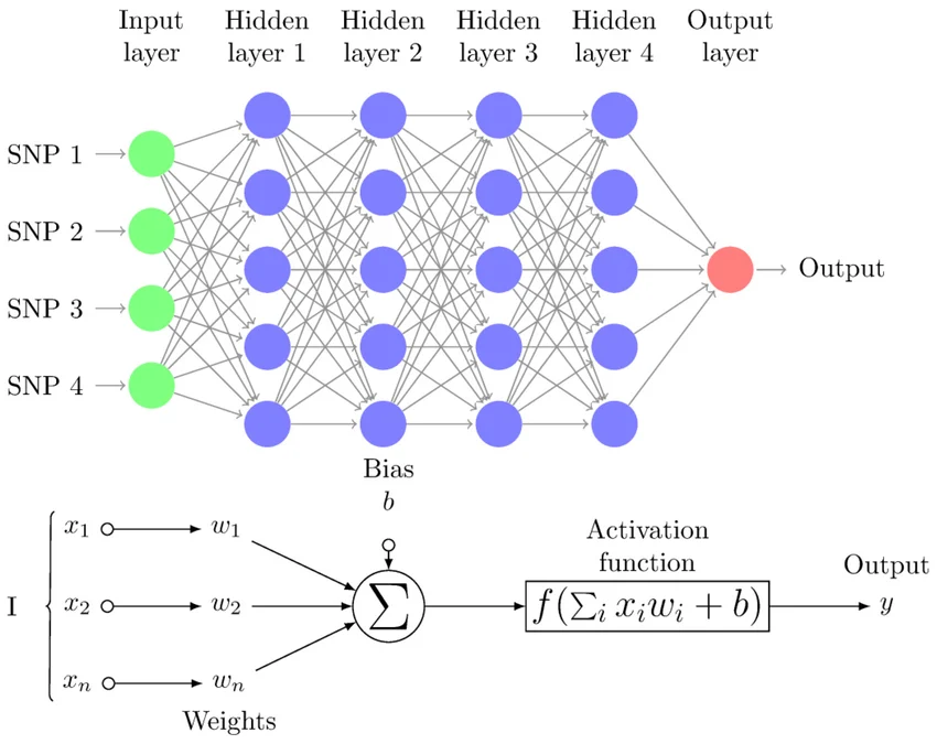
# note: Every neuron (except input neurons) has its own bias.
# the actual network has 21 different bias values.
# Hidden layer 1: 5 biases, Hidden layer 2: 5 biases, Hidden layer 3: 5 biases, Hidden layer 4: 5 biases, Output layer: 1 bias
# also: every arryw has a weight, the weight is not just for input neurons
#

Open original image: mlp.webp

# Earlier, we manually built expressions like:
#
#     e = a * b
#     d = e + c
#     L = d.tanh()
#
# and draw_dot(L) visualized that computation graph.
#
# With Neuron, Layer, and MLP, we no longer write those expressions ourselves.
# Instead, we simply call:
#
#     n(x)
#
# where x is the input data (e.g. [2.0, 3.0, -1.0]).
#
# Although n(x) looks like a single function call, it actually performs many
# Value operations internally. For a neuron with three inputs, it is roughly
# equivalent to writing:
#
#     p1 = w1 * x1
#     p2 = w2 * x2
#     p3 = w3 * x3
#
#     s1 = p1 + p2
#     s2 = s1 + p3
#     s3 = s2 + b
#
#     out = tanh(s3)
#
# Every multiplication, addition, and tanh() creates a new Value object.
# Each Value stores references to the Value objects that created it (_prev),
# automatically building the computation graph as the forward pass executes.
#
# Therefore:
#
#     draw_dot(n(x))
#
# does NOT visualize the function call "n(x)" itself. It visualizes the hidden
# computation graph produced by all the Value operations that occurred while
# evaluating n(x). draw_dot() starts from the final output Value and follows
# the _prev links backwards, reconstructing the entire mathematical expression.
#
# The same idea extends to a Layer and an MLP. Calling
#
#     mlp(x)
#
# sequentially calls every layer, and each layer sequentially calls every neuron.
# Each neuron builds its own expression graph, whose outputs become the inputs to
# the next layer. By the time the final prediction is produced, one large connected
# computation graph has been created automatically, even though we only wrote:
#
#     output = mlp(x)
#
# This is why draw_dot(output) can visualize the entire neural network's forward
# computation without us ever manually writing the individual expressions.

draw_dot(n(x))

# notice that gradients for all of them is 0, cuz we only did a forward pass
# now lets do backpropagation here

Loss and gradient descent¶

# lets create a tiny dataset
xs = [
    [2.0, 3.0, -1.0],
    [3.0, -1.0, 0.5],
    [0.5, 1.0, 1.0],
    [1.0, 1.0, -1.0]
]
ys = [1.0, -1.0, -1.0, 1.0] # desired targets, i.e. we want the neural net to output 1.0 when [2.0, 3.0, -1.0] is fed, and so on for other outputs too.

# what does our neural net currently think of these examples?
ypred = [n(x) for x in xs]
ypred
# some we will want to push up, some push down, so how do we tune the weights to better predict the desired targets
# the trick used in deep learning is to calculate a single number that somehow measures the total performance of our neural net
# we call this single number the loss
# so we are going to define a single number: loss that basically measures how well the neural net is performing
# the loss will be high cuz obviously we are not meeting desired results randomly, and our goal is to minimize the loss
# in this particular example, we are going to implement the mean squared error loss

[Value (data=0.8126717366460746),
 Value (data=0.7736417670870228),
 Value (data=0.7155829626079588),
 Value (data=0.9297704830267638)]

# ygt: y ground truth(actual truth value set by us), yout: y output, the current output by neuralnet
# the zip iterates over tuples of ygt and yout
[(ygt - yout)**2 for ygt, yout in zip(ys, ypred)]
loss = sum([(ygt - yout)**2 for ygt, yout in zip(ys, ypred)])
loss

Value (data=6.12905408285177)

# we want to minimize loss now ofcourse, so let's do
loss.backward() #something magical shall happen

n.layers[0].neurons[0].w[0].grad

-0.04414672653498933

# we saw that the gradient is positive, so it's influence on the loss is positive, so slightly decreasing this particular weight of this neuron of this layer will reduce the loss

draw_dot(loss)

# gradients on input data are not significant to us, because input data are fixed and unchangeable, so we are not concerned with their gradients even though they exist
# we are interested with the gradients of weights and biases

# we want some convenient code that can help us gather all parameters of neural net and operate on them simultaneously
# then we will nudge every parameter by a tiny amount based on the gradient information
# defined parameters method for a neuron

<__main__.MLP at 0x76eb026a56a0>

n.parameters()
len(n.parameters())

41

n.layers[0].neurons[0].w[0].grad
# this neuron's gradient is slightly negative

-0.04414672653498933

# current value of this neuron
n.layers[0].neurons[0].w[0].data

0.701533678275561

# now we want to slightly change the parameters(weights,biases) according to the gradient information
# gradient descent: gradient: vector/n-dimensional slope pointing in the direction of increased loss
# why do we want to set the stepsize as negative? we want to decrease the loss
# eg. for neuron with data 0.701533, its grad is negative, that means to decrease the value of this neuron we need to move along the direction of gradient, i.e. decrease it in this case
# generally gradient descent points to the direction of increasing the loss, but since we want to decrease the loss instead, we move in the opposite direction

for p in n.parameters():
    p.data += (-0.01) * p.grad

n.layers[0].neurons[0].w[0].data
# note that this value increased

0.7019751455409109

# let's reevaluate the loss
ypred = [n(x) for x in xs]
loss = sum([(ygt - yout)**2 for ygt, yout in zip(ys, ypred)])
loss
# from a cell up above, the loss that time was: Value (data=6.12905408285177), we hope our new loss is lower this time

Value (data=5.786701829767263)

# this way, we are doing gradient descent optimization manually, we do a loss.backward again
loss.backward()

for p in n.parameters():
    p.data += (-0.01) * p.grad

# let's reevaluate the loss
ypred = [n(x) for x in xs]
loss = sum([(ygt - yout)**2 for ygt, yout in zip(ys, ypred)])
loss
# from a cell up above, the loss that time was: Value (data=5.786701829767263), we hope our new loss is lower this time

Value (data=4.953693919118485)

loss.backward()
for p in n.parameters():
    p.data += (-0.01) * p.grad
# let's reevaluate the loss
ypred = [n(x) for x in xs]
loss = sum([(ygt - yout)**2 for ygt, yout in zip(ys, ypred)])
loss

Value (data=3.502461447115042)

loss.backward()
for p in n.parameters():
    p.data += (-0.01) * p.grad
# let's reevaluate the loss
ypred = [n(x) for x in xs]
loss = sum([(ygt - yout)**2 for ygt, yout in zip(ys, ypred)])
loss

Value (data=2.19299253743404)

loss.backward()
for p in n.parameters():
    p.data += (-0.01) * p.grad
# let's reevaluate the loss
ypred = [n(x) for x in xs]
loss = sum([(ygt - yout)**2 for ygt, yout in zip(ys, ypred)])
loss

Value (data=1.2758915302474378)

ypred

[Value (data=-0.32449875003546297),
 Value (data=-0.9236835702546978),
 Value (data=-0.8555744637945119),
 Value (data=0.3811903341108977)]

loss.backward()
for p in n.parameters():
    p.data += (-0.01) * p.grad
# let's reevaluate the loss
ypred = [n(x) for x in xs]
loss = sum([(ygt - yout)**2 for ygt, yout in zip(ys, ypred)])
loss

Value (data=0.5191358455506375)

loss.backward()
for p in n.parameters():
    p.data += (-0.01) * p.grad
# let's reevaluate the loss
ypred = [n(x) for x in xs]
loss = sum([(ygt - yout)**2 for ygt, yout in zip(ys, ypred)])
loss

Value (data=0.03662082713803008)

ypred # the predictions are now much closer

[Value (data=0.8185809216684239),
 Value (data=-0.9781569187143231),
 Value (data=-0.9438152648250223),
 Value (data=0.991391835932298)]

# if your learning rate is too low, it will take long time to converge
# but if its too high, the whole thing gets unstable and the loss might explode
# finding a subtle step size is an art

loss.backward()
for p in n.parameters():
    p.data += (-0.01) * p.grad
# let's reevaluate the loss
ypred = [n(x) for x in xs]
loss = sum([(ygt - yout)**2 for ygt, yout in zip(ys, ypred)])
loss

Value (data=8.476497401128291e-05)

# we got a really nice result, now our prediction is very close to our actual desired data
ypred

[Value (data=0.999620202267521),
 Value (data=-0.997202238808908),
 Value (data=-0.9912466841367535),
 Value (data=0.9995844023465608)]

# do it again and again, do a forward pass, backward pass, and update until loss is very less or you exceed the number of iterations
# be careful about selecting a step size too high which can result in overshooting and destabilize training

# now we have to iterate this process until desired scores are obtained

n.parameters() # the settings of weights and biases that makes our network predict the desired targets, and we've successfully trained a neural net

[Value (data=0.8088518819355177),
 Value (data=-0.7377474350651416),
 Value (data=0.9289440446884769),
 Value (data=-0.40062213654752804),
 Value (data=0.6422877552639026),
 Value (data=-0.40941960708816333),
 Value (data=0.531432679732588),
 Value (data=-0.5700844501926393),
 Value (data=0.5806905900555772),
 Value (data=-0.18085872399536607),
 Value (data=1.6621816874144193),
 Value (data=-0.712127047333736),
 Value (data=-0.06611187690607105),
 Value (data=-0.3213291670060825),
 Value (data=1.4383849020011432),
 Value (data=1.3394165145261139),
 Value (data=1.1912081375390375),
 Value (data=0.7819231331962886),
 Value (data=0.7526304327237721),
 Value (data=0.9050518483372895),
 Value (data=0.03087352613880031),
 Value (data=0.5190130231609394),
 Value (data=0.9757681460648503),
 Value (data=1.7853780339290244),
 Value (data=0.5798906051385159),
 Value (data=0.7332032613669759),
 Value (data=0.3711451212034126),
 Value (data=-0.9131118393783689),
 Value (data=1.0116802510598324),
 Value (data=0.34070381401402955),
 Value (data=-0.5112225059827382),
 Value (data=-1.0654026139897113),
 Value (data=-0.511363490778174),
 Value (data=-0.1568804168464658),
 Value (data=0.07179914404016574),
 Value (data=0.30192389227364896),
 Value (data=-1.6286353724473421),
 Value (data=-0.9201454432507071),
 Value (data=-0.8790888407781438),
 Value (data=0.8066669261414844),
 Value (data=0.2084758624186683)]

# say we want input layer with 3 neurons, 2 hidden layers each having four neurons and an output unit

x = [2.0, 3.0, -1.0]
n = MLP(3, [4, 4, 1])# we want 3 inputs into 2 layers of 4 and one output
n(x)

# this is the forward pass of an MLP
# currently we have just a single element, but its wrapped in a list because Layer always returns a list
# so for convenience, return only  first element if only first element is present else return full list

Value (data=-0.8735856111739421)

# now lets implement an actual training loop
# lets create a tiny dataset
xs = [
    [2.0, 3.0, -1.0],
    [3.0, -1.0, 0.5],
    [0.5, 1.0, 1.0],
    [1.0, 1.0, -1.0]
]
ys = [1.0, -1.0, -1.0, 1.0] # desired targets,

for k in range(20):

    # forward pass
    ypred = [n(x) for x in xs]
    loss = sum([(ygt - yout)**2 for ygt, yout in zip(ys, ypred)])

    # backward pass
    for p in n.parameters():
        p.grad = 0.0
    loss.backward()

    # update: gradient descent
    for p in n.parameters():
        p.data += (-0.05) * p.grad

    print(k, loss.data, )

0 7.1510237915308235
1 6.649857831439435
2 5.5469600957745
3 3.495952575400155
4 2.2778283159059693
5 1.4694219996623783
6 0.9239611321292588
7 0.6032064669008367
8 0.4194582914005529
9 0.30786128642294985
10 0.23571573278669522
11 0.18648634257376526
12 0.1514939855461927
13 0.12584513551785426
14 0.10657196985070957
15 0.09177101325151531
16 0.08017596572781989
17 0.07092401482834695
18 0.0634163767418835
19 0.05723048088512438

ypred

[Value (data=0.9999999999138397),
 Value (data=-0.9504567985360031),
 Value (data=-0.9805216455095753),
 Value (data=0.9999999998546136)]

# there is actually a subtle bug (you forgot to .zero_grad() in pytorch before .backward())
# as you know, all weights and biases have a .data and a .grad, and .grad starts at zero
# then we do .backward(), then fill in the gradients, then we do an update(gradient descent) on the data
# but we don't flush the grad and it stays there
# so when we do the second forward pass and do the backward again, remember that all backward operations do a += on the grad
# so the gradients add up and never get reset to zero
# thus: we need to zero grad before backwards

# you may notice that descent happens slowly and that's fine
# the reason why the previous one worked (no reset of grad) was because this was a very very simple problem
# and it is very easy for this neural net to fit this data
# so the grads ended up accumulating and gave us a massive step size, thus we converged extremely fast
# so now we have to do lots of steps to get a very low value of loss

draw_dot(loss)

# working with neural nets is tricky because your neural net might work just like ours worked with bugs
# but if the problem was complex, the loss wouldn't have been optimized very well

# now we summarize what we've learnt
# what are neural nets?
# neural nets are the mathematical expressions (fairly simple mathematical expressions in case of MLP) that take input as data, weights and bias of neural net,
# mathematical expression for the forward pass followed by a loss function(tries to measure accuracy of predictions)
# we backward the loss, use backpropagation to get the gradient, then we tune all the parameters to decrease the loss locally
# but we have to iterate this process many times and it's called the gradient descent, simply follow the gradient information
# we can have billions/trillions of parameters and get them to do whatever we want

# in case of gpt, we have massive amounts of text from the internet, and we're trying to make the neural net to predict the next word by taking a few words as input
# in that case the surface level concept is the same, but inner implementation differs
# eg. loss function would not be mean square error, it would be cross-entropy loss for predicting the next token
# there is not that much difference in using non-linearity for tanh, relu or sigmoid functions

# learning rate decay
# learning rate scaled based on number of iterations, learning rate shrinks as the network stabilizes to get the fine details

Reflections: Artificial vs. Biological Learning Building Micrograd from scalar first-principles clarifies exactly how modern neural networks learn, but it also highlights the stark contrast between machine learning and biological nervous systems.

The Weight Transport Problem: Micrograd relies on backpropagation, which requires the backward pass to use the exact same weight values as the forward pass (self.grad += out.grad * other.data). In a physical nervous system, there is no known mechanism for exact symmetric weight transport. How biology approximates this remains an open question.

Global vs. Local Learning Rules: Backpropagation requires a global error signal (the loss) to be routed backward through the entire computational graph. Biological systems are highly distributed and rely primarily on local learning rules (e.g., Hebbian learning or Spike-Timing-Dependent Plasticity), where weight updates depend only on the activity of the two adjacent neurons.

Continuous vs. Spiking: Micrograd uses continuous scalar values and non-linear activation functions like tanh. Biological systems communicate via discrete, asynchronous electrical pulses (spikes).