Building a decoder transformer
Original study notes by Satish Bajagain, following Andrej Karpathy’s Zero to Hero. Comments, intermediate attempts and saved outputs are retained. Section titles are navigation additions.
Reading note · 10 October 2026. This lesson and its character-level GPT implementation are complete. Original attempts and outputs are preserved. Before reusing the accompanying transformer script, read the attention-scaling correction; the correction is separate from the archived code.
Text, tokens and training data
# in our case, output will be character by character, but in chatgpt's case, output is coming out token by token
# a token is not word level but more of a word chunk level
# we'll download the tiny shakespeare dataset to train on
!wget https://raw.githubusercontent.com/karpathy/char-rnn/master/data/tinyshakespeare/input.txt--2026-09-12 19:31:45-- https://raw.githubusercontent.com/karpathy/char-rnn/master/data/tinyshakespeare/input.txt
Resolving raw.githubusercontent.com (raw.githubusercontent.com)... 2606:50c0:8002::154, 2606:50c0:8000::154, 2606:50c0:8001::154, ...
Connecting to raw.githubusercontent.com (raw.githubusercontent.com)|2606:50c0:8002::154|:443... connected.
HTTP request sent, awaiting response... 200 OK
Length: 1115394 (1.1M) [text/plain]
Saving to: ‘input.txt.5’
input.txt.5 100%[===================>] 1.06M --.-KB/s in 0.1s
2026-09-12 19:31:46 (7.17 MB/s) - ‘input.txt.5’ saved [1115394/1115394]
# read the input file
with open('input.txt', 'r', encoding='utf-8') as f:
    text = f.read()
print(len(text)) #we're working with roughly 1 million characters
1115394
# to look at the first 100 characters
print(text[:100])
# this text is just a sequence of characters
First Citizen:
Before we proceed any further, hear me speak.
All:
Speak, speak.
First Citizen:
You
chars = sorted(list(set(text))) # why set? to get just unique chars, why list?: for ordering purposes(sets are unordered), sorted?: ensure proper ordering
vocab_size = len(chars)
print(''.join(chars))
print(vocab_size)
 !$&',-.3:;?ABCDEFGHIJKLMNOPQRSTUVWXYZabcdefghijklmnopqrstuvwxyz
65
# we want to develop some strategy to tokenize the input text
# tokenize: means to convert the raw text as a string to some sequence of integers acc to some vocabulary of possible elements
# since we're building a character level language model, we translate individual characters into integers
# create a mapping from characters to integers
itos = {i: ch for i, ch in enumerate(chars)}
stoi = {ch: i for i, ch in enumerate(chars)}
encode = lambda s: [stoi[c] for c in s] #encoder: take a string, output a list of integers
decode = lambda l: ''.join([itos[i] for i in l]) #decoder: take a list of integers, output a string
print(encode("sup bro"))
print(decode(encode("sup bro")))[57, 59, 54, 1, 40, 56, 53]
sup bro
# but this is just one of many possible encoding/tokenizers, but there are a lot of other alternatives
# eg. google uses SentencePiece: encode text into integers in a diff schema using diff vocabulary, and is a sub-word tokenizer(not char-level, nor word-level, but sub-word level)
# this sub-word level is what's done in practice
# openai's library: tiktoken, uses byte pair encoding tokeniser
import tiktoken
enc = tiktoken.get_encoding('gpt2')
print(enc.n_vocab) #our earlier example: we had 65 tokens A-Za-zetc, but here its 50k+ tokens50257
# and when we encode the exact same stuff
print(enc.encode("sup bro"))
print(enc.decode(enc.encode("sup bro")))
[37330, 1379]
sup bro
# that tiktoken was a small eg, we're sticking with our own encoder/decoder for simplicity
# we can now tokenize the entire training set of shakespeare cuz we have our encoder and decoder functions
# encode entire text dataset, and store it into a Torch.tensor
import torch
data = torch.tensor(encode(text), dtype=torch.long) #encode all text and wrap it into torch.Tensor
print(len(encode(text)))
print(data.shape, data.dtype)
print(data[:100]) #same as prev but encoded and in a tensor1115394
torch.Size([1115394]) torch.int64
tensor([18, 47, 56, 57, 58, 1, 15, 47, 58, 47, 64, 43, 52, 10, 0, 14, 43, 44,
53, 56, 43, 1, 61, 43, 1, 54, 56, 53, 41, 43, 43, 42, 1, 39, 52, 63,
1, 44, 59, 56, 58, 46, 43, 56, 6, 1, 46, 43, 39, 56, 1, 51, 43, 1,
57, 54, 43, 39, 49, 8, 0, 0, 13, 50, 50, 10, 0, 31, 54, 43, 39, 49,
6, 1, 57, 54, 43, 39, 49, 8, 0, 0, 18, 47, 56, 57, 58, 1, 15, 47,
58, 47, 64, 43, 52, 10, 0, 37, 53, 59])
# so now, the entire dataset of text is re-represented/stretched out as a single very large sequence of integers# we want to separate/split our dataset into training and validation sets
n = int(0.9 * len(data)) #first 90% will be train, rest 10% will be val
train_data = data[:n]
val_data = data[n:]
# its purpose: to help us understand, to what extent our model is overfitting, we're hiding the validation data for now
# cuz we don't want an exact memorization of the exact Shakespeare
# we want a neural network that creates a shakespeare like text# we now want to start plugging in these integer sequences into transformer
# so that it can train and learn those patterns
# we'll never feed the entire text into a transformer all at once
# cuz that would be very computationally expensive
# so when we train transformer with the datasets, we work with only chunks of the dataset
# and when we train the transformer, we sample random little chunks out of training set,
# and train on just chunks at a time, and these chunks have a maximum length
# we refer to this maximum length of a chunk as block_size or context_lengthblock_size = 8
train_data[:block_size+1] #why +1? lets look at the first 9 characters in the training set
# note: when we sample a chunk of data, this actually has way more example packed into it cuz all characters follow each othertensor([18, 47, 56, 57, 58, 1, 15, 47, 58])# when we plug this chunk into a transformer,
# we simultaneously train it to make prediction at every one of these positions
# there are 8 examples in a chunk of 9 characters, so for block_size=8 above, we took block_size + 1 characters for training data
# eg 1. 18 -> 47, i.e. given context of 18, 47 likely comes next
# eg 2. 18 47 -> 56, i.e. given context of 18 47, 56 likely comes next
# thus there are 8 examples, for each one of these examples: 47 - 58 is output.# we want to illustrate that same example with code
x = train_data[:block_size] #inputs to the transformer
y = train_data[1:block_size + 1] #y: offset by 1, cuz y: targets for each position in input
for t in range(block_size):
context = x[:t+1] #context is always all characters upto t and including t, ah yes, initially t=0, t+1 confused me
target = y[t]
print(f"when input is {context} the target: {target}")when input is tensor([18]) the target: 47
when input is tensor([18, 47]) the target: 56
when input is tensor([18, 47, 56]) the target: 57
when input is tensor([18, 47, 56, 57]) the target: 58
when input is tensor([18, 47, 56, 57, 58]) the target: 1
when input is tensor([18, 47, 56, 57, 58, 1]) the target: 15
when input is tensor([18, 47, 56, 57, 58, 1, 15]) the target: 47
when input is tensor([18, 47, 56, 57, 58, 1, 15, 47]) the target: 58
# Train on contexts from 1 up to block_size, not just for efficiency.
# This teaches the Transformer to handle any context length during inference.
# During generation, context can grow from 1 → block_size.
# Beyond block_size, truncate the context since the model never sees longer inputs.
Batches and prediction targets
torch.manual_seed(1337) #since we're gonna sample random locations in dataset to pull chunks from, setting seed in rng ensures same result for andrej and me
batch_size = 4 #how many independent sequences will we process in parallel in every forward/backward pass of transformer?
block_size = 8 #what is the maximum context length for predictions?

def get_batch(split):
    # generate a small batch of data of inputs x and targets y
    data = train_data if split == 'train' else val_data
    ix = torch.randint(len(data) - block_size, (batch_size, )) #generate batch_size number of random offsets, and since batch_size = 4, ix will be 4 randomly generated numbers betn 0 and len(data) - block_size
    x = torch.stack([data[i: i + block_size] for i in ix])
    y = torch.stack([data[i+1: i+block_size+1] for i in ix])
    return x, y

xb, yb = get_batch('train')
print('inputs:')
print(xb.shape)
print(xb)
print('targets:')
print(yb.shape)
print(yb)

print('---')

for b in range(batch_size): #batch_dimension
    for t in range(block_size): #time_dimension
        context = xb[b, :t+1]
        target = yb[b, t]
        print(f"when input is {context.tolist()} the target: {target}")
inputs:
torch.Size([4, 8])
tensor([[24, 43, 58, 5, 57, 1, 46, 43],
[44, 53, 56, 1, 58, 46, 39, 58],
[52, 58, 1, 58, 46, 39, 58, 1],
[25, 17, 27, 10, 0, 21, 1, 54]])
targets:
torch.Size([4, 8])
tensor([[43, 58, 5, 57, 1, 46, 43, 39],
[53, 56, 1, 58, 46, 39, 58, 1],
[58, 1, 58, 46, 39, 58, 1, 46],
[17, 27, 10, 0, 21, 1, 54, 39]])
---
when input is [24] the target: 43
when input is [24, 43] the target: 58
when input is [24, 43, 58] the target: 5
when input is [24, 43, 58, 5] the target: 57
when input is [24, 43, 58, 5, 57] the target: 1
when input is [24, 43, 58, 5, 57, 1] the target: 46
when input is [24, 43, 58, 5, 57, 1, 46] the target: 43
when input is [24, 43, 58, 5, 57, 1, 46, 43] the target: 39
when input is [44] the target: 53
when input is [44, 53] the target: 56
when input is [44, 53, 56] the target: 1
when input is [44, 53, 56, 1] the target: 58
when input is [44, 53, 56, 1, 58] the target: 46
when input is [44, 53, 56, 1, 58, 46] the target: 39
when input is [44, 53, 56, 1, 58, 46, 39] the target: 58
when input is [44, 53, 56, 1, 58, 46, 39, 58] the target: 1
when input is [52] the target: 58
when input is [52, 58] the target: 1
when input is [52, 58, 1] the target: 58
when input is [52, 58, 1, 58] the target: 46
when input is [52, 58, 1, 58, 46] the target: 39
when input is [52, 58, 1, 58, 46, 39] the target: 58
when input is [52, 58, 1, 58, 46, 39, 58] the target: 1
when input is [52, 58, 1, 58, 46, 39, 58, 1] the target: 46
when input is [25] the target: 17
when input is [25, 17] the target: 27
when input is [25, 17, 27] the target: 10
when input is [25, 17, 27, 10] the target: 0
when input is [25, 17, 27, 10, 0] the target: 21
when input is [25, 17, 27, 10, 0, 21] the target: 1
when input is [25, 17, 27, 10, 0, 21, 1] the target: 54
when input is [25, 17, 27, 10, 0, 21, 1, 54] the target: 39
# Batch dimension = number of independent sequences/chunks processed in parallel.
# It is mainly for efficiency: GPUs are good at parallel processing.
# Each batch row is processed independently; sequences in different rows do NOT interact.

# batch_size = 4 → process 4 independent sequences per forward/backward pass.
# block_size = 8 → maximum context length used to predict the next token.

# get_batch():
#   - Randomly choose batch_size offsets into the dataset.
#   - For each offset i:
#       x = data[i : i + block_size]       # input sequence
#       y = data[i+1 : i + block_size+1]   # same sequence shifted by 1 → targets
#   - torch.stack() stacks the sequences into a (batch_size, block_size) tensor.
#   - Therefore xb and yb have shape (4, 8): 4 independent chunks × 8 time positions.

# A (B, T) tensor contains B × T independent training examples.
# Here: 4 × 8 = 32 input→target prediction examples packed into one batch.

# For each batch b and time t:
#   context = xb[b, :t+1]  # progressively growing context within that sequence
#   target = yb[b, t]      # correct next token for that context
# The Transformer processes all 4 sequences and all positions simultaneously.
# The targets yb provide the correct answer at every position for computing the loss.
print(xb) #we now have our batch of input that we want to feed to our transformer, let's feed it to neural networkstensor([[24, 43, 58, 5, 57, 1, 46, 43],
[44, 53, 56, 1, 58, 46, 39, 58],
[52, 58, 1, 58, 46, 39, 58, 1],
[25, 17, 27, 10, 0, 21, 1, 54]])
# we'll start with simplest possible neural network which in the case of language modeling is the Bigram language model
# following is the pytorch module that implements the bigram language model
A bigram baseline
import torch
import torch.nn as nn
from torch.nn import functional as F
torch.manual_seed(1337)

# constructing a Bigram language model which is a subass of NN module
class BigramLanguageModel(nn.Module):

    def __init__(self, vocab_size):
        super().__init__()
        # each token directly reads off the logits for the next token from a lookup table
        self.token_embedding_table = nn.Embedding(vocab_size, vocab_size)
        # nn.Embedding() is a very thin wrapper around a tensor of shape vocab_size x vocab_size

    def forward(self, idx, targets):

        # idx and targets are both (B,T) tensors of integers
        logits = self.token_embedding_table(idx) # (B,T,C) #when we pass idx here,
        # each idx in our input will refer the embedding table xb above, and pluck a row out of that embedding table corresponding to its index
        # eg. 24 will go to the embedding table and pluck out the 24th row, then 43 will go and pluck out 43rd row and so on
        # pytorch will arrange all of this into a Batch by Time by Channel tensor, C = vocab_size
        # simply, we pluck out rows and then arrange them in a BXTXC, they are interpreted as logits:(scores for next characters in the sequence)
        # currently the tokens are not talking to each other / not seeing any context,
        # we're predicting what comes next just based on the individual identity of a single token
        # currently, a token knows what comes next just by knowing what token it is cuz certain characters follow other characters

        # by running the above cell, we got the predictions/scores for every one of the 4x8 positions about what comes next
        # now we want to evaluate the loss function: use negative log likelihood loss (in makemore), in pytorch nll is under the name cross_entropy

        B,T,C = logits.shape #unpack the numbers
        logits = logits.view(B*T, C) #2-D array
        # stretch out all positions in a 1-dimensional sequence and preserve channel dimension as second dimension, so we stretched it out into 2 dimensions
        # we also have to do the same with targets, cuz currently targets are of shape BxT but we want it to be 1D i.e. B*T
        targets = targets.view(B*T) #targets.view(-1) also works as pytorch will figure out the same, but better to be as explicit as possible

        loss = F.cross_entropy(logits, targets) #measures quality of logits w.r.t target, i.e. how well are we predicting the next character based on logits
        # optimally, the correct dimension of logits (based on target) should be very high, and all other dimensions should be very low
        # but obviously, this won't be so initially
        return logits, loss

# m = BigramLanguageModel(vocab_size)
# logits, loss = m(xb, yb)
# print(logits.shape, loss)

# why did we get the error? if you look at pytorch documentation
# https://docs.pytorch.org/docs/2.13/generated/torch.nn.functional.cross_entropy.html
# it expects inputs in the form of (N,C,d1,d2,...,dK), i.e. channels in middle, but we instead have BxTxC
# so we need to reshape our logits

m = BigramLanguageModel(vocab_size)
logits, loss = m(xb, yb)
print(logits.shape, loss)
torch.Size([32, 65]) tensor(4.8786, grad_fn=<NllLossBackward0>)
# our loss is currently: 4.87, our vocab_size=65, we can guess what the loss should be since we studied negative log likelihood before
# we're expecting -ln(1/65) = 4.174387
# this difference tells us that the initial predictions are not super diffuse, they've got entropy so we're guessing wrong
# we saw how to evaluate quality of model, now we want to see how to generate from the model
import torch
import torch.nn as nn
from torch.nn import functional as F
torch.manual_seed(1337)
class BigramLanguageModel(nn.Module):
def __init__(self, vocab_size):
super().__init__()
self.token_embedding_table = nn.Embedding(vocab_size, vocab_size)
def forward(self, idx, targets=None):
logits = self.token_embedding_table(idx) # (B,T,C) #when we pass idx here,
if targets is None:
loss = None
else:
B,T,C = logits.shape #unpack the numbers
logits = logits.view(B*T, C) #2-D array
targets = targets.view(B*T) #targets.view(-1) also works as pytorch will figure out the same, but better to be as explicit as possible
loss = F.cross_entropy(logits, targets)
return logits, loss
def generate(self, idx, max_new_tokens):
# idx is (B,T) array of indices in the current context of some characters in a batch
for _ in range(max_new_tokens):
logits, loss = self(idx) #get the predictions
logits = logits[:, -1, :] #focus only on the last time step # becomes (B,C)
probs = F.softmax(logits, dim=1) #apply softmax to get probabilities # (B,C)
idx_next = torch.multinomial(probs, num_samples=1) #sample from the distribution #(B,1)
idx = torch.cat((idx, idx_next), dim=1) #append sampled index to the running sequence #(B, T+1)
return idx
m = BigramLanguageModel(vocab_size)
logits, loss = m(xb, yb)
print(logits.shape, loss)
# print(decode(m.generate(torch.zeros((1,1), dtype=torch.long), max_new_tokens=100)[0].tolist()))
# idx = torch.zeros((1,1), dtype=torch.long) #creating a 1x1 tensor with batch and time 1-d, all values 0 (more like single value 0)
# note from above that 0 = \n probably, so its reasonable to feed in as the very first character in a sequence
# print(decode(m.generate(idx), max_new_tokens=100)[0].tolist())
print(decode(m.generate(torch.zeros((1,1), dtype=torch.long), max_new_tokens=100)[0].tolist()))
# since generate() works on the level of batches, we have to index into the 0th row to unplug the single batch dimension that exists
# then it gives us time steps: just a 1D array of all indices which we will convert to list from pytorch tensor
# then feed it into our decode function and convert those integers into texttorch.Size([32, 65]) tensor(4.8786, grad_fn=<NllLossBackward0>)
SKIcLT;AcELMoTbvZv C?nq-QE33:CJqkOKH-q;:la!oiywkHjgChzbQ?u!3bLIgwevmyFJGUGp
wnYWmnxKWWev-tDqXErVKLgJ
# create a pytorch optimization object
# we're using the AdamW optimizer, in makemore we only used stochastic gradient descent: simplest possible optimizer: you can replace AdamW with SGD
# AdamW is much more advanced and popular than SGD
# a good learning rate is actually lower, but for very small networks, we can get away with much higher learning rates
optimizer = torch.optim.AdamW(m.parameters(), lr=1e-3)
# the optimizer object will take the gradients and update the parameters using the gradients
batch_size = 32
# our training loop
for steps in range(19000):
# sample a batch of data
xb, yb = get_batch('train')
# evaluate the loss
logits, loss = m(xb, yb)
optimizer.zero_grad(set_to_none=True) #zeroing out the gradients from the previous step
loss.backward() #getting the gradients for all the parameters
optimizer.step() #using those gradients to update our parameter
print(loss.item())2.5222437381744385
print(decode(m.generate(torch.zeros((1,1), dtype=torch.long), max_new_tokens=100)[0].tolist()))
# we're expecting this output to be somewhat reasonable
NGRDoome dir hay modo
ILISust h t ar o ct wis atino g;
Pomarth thapes n allly s;
ARIARYof tol-Hison
print(decode(m.generate(torch.zeros((1,1), dtype=torch.long), max_new_tokens=300)[0].tolist()))
# we're expecting this output to be somewhat reasonable
IZAff: buinenod r d bl, I myondstheat
Surs hanishosigre Whond d y w is to s ans nga omastathest hy nor t ty or,
PEre wat vemesthemarongy th n:
Wr cate 'sshand astt t:
G sanond s, Wharit hencolcle nd de yosteled itis w s.

TRI baror.
SABy by
LO 'd; m therdse.
ORCHelouror:
Rilld ss atidrrs urenathty h
# we got a little progress, progress is progress, but still not shakespeare# this is a very simple model cuz the tokens are not talking to each other
# so for whatever was generated, we're only looking at the very last character to make the prediction about what comes next
# so, now the tokens have to start talking with one another and figure out what is in the context to make better predictions
# now we focus on the transformer partRecorded baseline training
# # we summarized everything into a bigram.py script and ran basically the same stuff there
# # heres the output:
# (.venv) bajagainsatish@HP-Pavilion:~/Anaconda Scripts/Andrej Karpathy$ python bigram.py
# step 0: train loss 4.7305, val loss 4.7241
# step 300: train loss 2.8110, val loss 2.8249
# step 600: train loss 2.5434, val loss 2.5682
# step 900: train loss 2.4932, val loss 2.5088
# step 1200: train loss 2.4863, val loss 2.5035
# step 1500: train loss 2.4665, val loss 2.4921
# step 1800: train loss 2.4683, val loss 2.4936
# step 2100: train loss 2.4696, val loss 2.4846
# step 2400: train loss 2.4638, val loss 2.4879
# step 2700: train loss 2.4738, val loss 2.4911

# MARI he avayokis erceller thour d, myono thishe me tord se by he me, Forder anen: at trselorinjulour t yoru thrd wo ththathy IUShe bavidelanoby man ond be jus as g e atot Meste hrle s, ppat t JLENCOLIUS:
# Oppid tes d s o ged moer y pevehear soue maramapay fo t: bueyo malalyo!
# Duir.
# Fl ke it I t l o'ddre d ondu s?
# cr, havetrathackes w.
# PUpee meshancun, hrendspouthoulouren whel's'sesoread pe, s whure our heredinsethes; sedsend r lo pamit,
# QUMIVIVIOfe m ne RDINid we tr ort; t:
# MINENXI l dintandore r
# (.venv) bajagainsatish@HP-Pavilion:~/Anaconda Scripts/Andrej Karpathy$
# we're almost ready to write our very own self-attention block to process the tokens
# but before that we want to get used to a mathematical trick used in self-attention inside a transformer
# it is at the heart of an efficient implementation of self-attention
# we'll work with a toy example to get used to this operation and it will be much clear laterThe mathematical trick in attention
The mathematical trick in self-attention:# consider the toy example:
torch.manual_seed(1337)
B,T,C = 4,8,2 #batch, time, channels(some info at each point in the sequence)
x = torch.randn(B,T,C)
x.shapetorch.Size([4, 8, 2])# we have 8 tokens in a batch, and these 8 tokens are not talking to each other
# but we want them to talk with one another, we'd like to couple them
# and we want to couple them in a very specific way,
# eg. the token at 5th location should not communicate with the token in 6th, 7th location cuz those are future tokens in sequence
# the token at 5th location should only talk to 4th, 3rd, 2nd and 1st token
# simply: we can't get any information from the future, because we're trying to predict the future
# so what is the easiest way for tokens to communicate?
# eg. if i am a 5th token, and i'd like to communicate with the past, the simplest way to do that is to just do an average of all the preceding elements
# ask ai to summarize from kinda 44:00 or something to 45:00# we want x[b, t] = mean_{i<=t} x[b, i]
# bow: bag of words: a term used when we're averaging up things: we're averaging up words stored on every one of these 8 locations
xbow = torch.zeros((B,T,C))
for b in range(B):
for t in range(T):
xprev = x[b, :t+1] # (t, C) #previous tokens are at the batch dimension b and everything upto the t'th token
xbow[b, t] = torch.mean(xprev, 0) #averaging out over the mean/0th dimension: over time, we'll get a 1d vector: C, which we'll store in bag of wordsx[0]tensor([[ 0.1808, -0.0700],
[-0.3596, -0.9152],
[ 0.6258, 0.0255],
[ 0.9545, 0.0643],
[ 0.3612, 1.1679],
[-1.3499, -0.5102],
[ 0.2360, -0.2398],
[-0.9211, 1.5433]])xbow[0]tensor([[ 0.1808, -0.0700],
[-0.0894, -0.4926],
[ 0.1490, -0.3199],
[ 0.3504, -0.2238],
[ 0.3525, 0.0545],
[ 0.0688, -0.0396],
[ 0.0927, -0.0682],
[-0.0341, 0.1332]])# compare xbow vs x, you'll see that for each component of xbow, it is average of all previous ones, and its values look much better/average
# the last one is averaging up of all the tokens
# this is good but inefficient
# continue from 47:12 but before that summarize some stuff at time 44:00 and add comment above# ============================================================
# GENERATION: WHAT generate() DOES
# ============================================================
# generate() takes the current context `idx` of shape (B, T)
# and repeatedly extends it with newly sampled tokens:
#
# (B, T) -> (B, T+1) -> (B, T+2) -> ...
#
# It generates `max_new_tokens` tokens while preserving the
# batch dimension, so every sequence in the batch is generated
# independently but in parallel.Understanding generation
# def generate(self, idx, max_new_tokens):
# # `idx` = current context of token indices, shape (B, T)
# # We repeatedly predict the next token and append it to idx.
# for _ in range(max_new_tokens):
# # Run the current context through the model.
# # No targets are provided because during generation we
# # don't have ground-truth answers and therefore don't
# # need to calculate a loss.
# logits, loss = self(idx)
# # logits has shape (B, T, C), containing predictions for
# # every position in every sequence.
# # We only care about the prediction at the LAST time step,
# # because that prediction tells us what token should come next.
# # (B, T, C) -> (B, C)
# logits = logits[:, -1, :]
# # Convert the logits for the next token into probabilities.
# # Each row now represents a probability distribution over
# # the vocabulary.
# probs = F.softmax(logits, dim=1) # (B, C)
# # Randomly sample ONE token from each probability distribution.
# # This gives the next token for every sequence in the batch.
# # (B, C) -> (B, 1)
# idx_next = torch.multinomial(probs, num_samples=1)
# # Append the newly sampled token to the existing sequence.
# # (B, T) + (B, 1) -> (B, T+1)
# idx = torch.cat((idx, idx_next), dim=1)
# return idx# ============================================================
# WHY targets=None IS IMPORTANT
# ============================================================
# During training:
# self(idx, targets)
# -> calculate logits AND loss
#
# During generation:
# self(idx)
# -> we only need logits; there are no ground-truth targets.
#
# Therefore `targets` must be optional.
# If targets is None, skip the loss calculation and return:
# logits, None
#
# This allows the same forward() function to work for both
# training and generation.# ============================================================
# STARTING GENERATION
# ============================================================
# We start with a 1x1 tensor:
#
# torch.zeros((1, 1), dtype=torch.long)
#
# Shape:
# B = 1 -> one sequence
# T = 1 -> one starting token
#
# The value 0 represents '\n' in this vocabulary, so it is used
# as a reasonable starting character for generation.
#
# generate(..., max_new_tokens=100) then repeatedly adds
# 100 new tokens to this initial context.
#
# After generation:
# [0, token1, token2, ..., token100]
#
# Since generate() keeps the batch dimension, we use [0] to
# select the first (and only) sequence:
#
# m.generate(...)[0]
#
# Then:
# .tolist()
# converts the PyTorch tensor into a normal Python list
#
# decode(...)
# converts the integer token IDs back into characters/text.# ============================================================
# WHY THE INITIAL OUTPUT IS GARBAGE
# ============================================================
# The model has NOT been trained yet.
#
# Its embedding table contains essentially random parameters,
# so its predictions are random as well.
#
# Therefore the generated text is expected to look like garbage.
#
# The next step is to TRAIN the model so that its probability
# distributions become meaningful and generation becomes less
# random.# ============================================================
# WHY GENERATE() FEEDS THE ENTIRE CONTEXT EVERY TIME
# ============================================================
# This implementation is intentionally GENERAL.
#
# For the current BigramLanguageModel, the prediction of the
# next character only depends on the immediately preceding
# character.
#
# Example:
# ... W -> K
#
# To predict K, the bigram model only needs W.
# Feeding the entire sequence is therefore unnecessary.
#
# However, later we will build models (e.g. Transformers) where
# the prediction DOES depend on the earlier history.
#
# Keeping generate() written this way means we don't have to
# rewrite it when the model becomes more powerful:
#
# current context
# ↓
# model predicts next token
# ↓
# sample token
# ↓
# append token to context
# ↓
# repeat
#
# So although this looks inefficient for a Bigram model, it is
# deliberately structured to work with future models that use
# the full context.# continue from 47:12# the above approach is very inefficient, and we can be very very efficient about doing that with matrix multiplicationtorch.manual_seed(42)
a = torch.ones(3,3)
b = torch.randint(0, 10, (3, 2)).float()
c = a @ b
print('a=')
print(a)
print('--')
print('b=')
print(b)
print('--')
print('c=') #3x3 x 3x2 => 3x2
print(c)
# because the rows in a's are all ones, in c notice that each element is the sum of columns of ba=
tensor([[1., 1., 1.],
[1., 1., 1.],
[1., 1., 1.]])
--
b=
tensor([[2., 7.],
[6., 4.],
[6., 5.]])
--
c=
tensor([[14., 16.],
[14., 16.],
[14., 16.]])
# tril: a PyTorch function that returns the lower triangular part of a matrix (2D tensor) or a batch of matrices# that all ones is boring, instead look at torch.tril
torch.tril(torch.ones(3, 3))tensor([[1., 0., 0.],
[1., 1., 0.],
[1., 1., 1.]])# so, what happens if we use this instead?
torch.manual_seed(42)
a = torch.tril(torch.ones(3,3))
b = torch.randint(0, 10, (3, 2)).float()
c = a @ b
print('a=')
print(a)
print('--')
print('b=')
print(b)
print('--')
print('c=') #3x3 x 3x2 => 3x2
print(c)
# because some values inside the rows in a's are zeros, some values in b get ignored,
# in c notice that each element is the sum of some columns of ba=
tensor([[1., 0., 0.],
[1., 1., 0.],
[1., 1., 1.]])
--
b=
tensor([[2., 7.],
[6., 4.],
[6., 5.]])
--
c=
tensor([[ 2., 7.],
[ 8., 11.],
[14., 16.]])
# currently, we're doing sums, but we can easily do an average as well if the values of row in 'a' sum to 1
# so normalize all rows so sum = 1torch.manual_seed(42)
a = torch.tril(torch.ones(3,3))
a = a / torch.sum(a, 1, keepdim=True)
b = torch.randint(0, 10, (3, 2)).float()
c = a @ b
print('a=')
print(a)
print('--')
print('b=')
print(b)
print('--')
print('c=') #3x3 x 3x2 => 3x2
print(c)
# because some values inside the rows in a's are zeros, some values in b get ignored,
# in c notice that each element is the sum of some columns of ba=
tensor([[1.0000, 0.0000, 0.0000],
[0.5000, 0.5000, 0.0000],
[0.3333, 0.3333, 0.3333]])
--
b=
tensor([[2., 7.],
[6., 4.],
[6., 5.]])
--
c=
tensor([[2.0000, 7.0000],
[4.0000, 5.5000],
[4.6667, 5.3333]])
# so by manipulating the elements of the multiplying matrix, and then multiplying it with any given matrix,
# we can do the averages in incremental fashion# now we see how we can vectorize this and make this more efficientwei = torch.tril(torch.ones(T, T))
wei = wei / wei.sum(1, keepdim = True)
weitensor([[1.0000, 0.0000, 0.0000, 0.0000, 0.0000, 0.0000, 0.0000, 0.0000],
[0.5000, 0.5000, 0.0000, 0.0000, 0.0000, 0.0000, 0.0000, 0.0000],
[0.3333, 0.3333, 0.3333, 0.0000, 0.0000, 0.0000, 0.0000, 0.0000],
[0.2500, 0.2500, 0.2500, 0.2500, 0.0000, 0.0000, 0.0000, 0.0000],
[0.2000, 0.2000, 0.2000, 0.2000, 0.2000, 0.0000, 0.0000, 0.0000],
[0.1667, 0.1667, 0.1667, 0.1667, 0.1667, 0.1667, 0.0000, 0.0000],
[0.1429, 0.1429, 0.1429, 0.1429, 0.1429, 0.1429, 0.1429, 0.0000],
[0.1250, 0.1250, 0.1250, 0.1250, 0.1250, 0.1250, 0.1250, 0.1250]])# this wei is how much we want to average up, its an avg cuz the rows sum to 1
# this wei is our 'a' from previous exampleWeighted aggregation
# consider the toy example:
torch.manual_seed(1337)
B,T,C = 4,8,2 #batch, time, channels(some info at each point in the sequence)
x = torch.randn(B,T,C)
x.shape
# we want x[b, t] = mean_{i<=t} x[b, i]
# bow: bag of words: a term used when we're averaging up things: we're averaging up words stored on every one of these 8 locations
xbow = torch.zeros((B,T,C))
for b in range(B):
    for t in range(T):
        xprev = x[b, :t+1] # (t, C) #previous tokens are at the batch dimension b and everything upto the t'th token
xbow[b, t] = torch.mean(xprev, 0) #averaging out over the mean/0th dimension: over time, we'll get a 1d vector: C, which we'll store in bag of wordswei = torch.tril(torch.ones(T, T))
wei = wei / wei.sum(1, keepdim = True)
xbow2 = wei @ x # (T,T) @ (B,T,C) ---> pytorch sees difference, and broadcasts by adding a Batch dimension as
# ---> (B, T, T) @ (B, T, C) --> so it'll apply matrix multiplication in all batch elements in parallely and individuall
# output ---> (B, T, C)
# torch.allclose(xbow, xbow2)
torch.allclose(xbow, xbow2, atol=1e-5)Truexbow[0], xbow2[0] #should be identical(tensor([[ 0.1808, -0.0700],
[-0.0894, -0.4926],
[ 0.1490, -0.3199],
[ 0.3504, -0.2238],
[ 0.3525, 0.0545],
[ 0.0688, -0.0396],
[ 0.0927, -0.0682],
[-0.0341, 0.1332]]),
tensor([[ 0.1808, -0.0700],
        [-0.0894, -0.4926],
        [ 0.1490, -0.3199],
        [ 0.3504, -0.2238],
        [ 0.3525,  0.0545],
        [ 0.0688, -0.0396],
        [ 0.0927, -0.0682],
[-0.0341, 0.1332]]))# so the trick here is: we were able to batch matrix multiply to do this aggregation,
# and its a weighted aggregation, and the weights are specified in this TxT array in lower triangular form, that aid the weighted sum
# it means that a token at 10th dimension will only get information from the tokens preceeding it
# finally, we want to rewrite it in one more way# version 3: use softmax
tril = torch.tril(torch.ones(T, T))
print(tril)
wei = torch.zeros((T, T)) #tells us: how much of each token from the past do we want to aggregate/average up
print(wei)
wei = wei.masked_fill(tril == 0, float('-inf')) #tokens from the future cannot communicate
print(wei)
wei = F.softmax(wei, dim=1) # a normalization operation, we exponentiate every single one of the values and divide by their sum
print(wei)
xbow3 = wei @ x
torch.allclose(xbow, xbow3, atol=1e-5)
# you can do weighted aggregations of your past elements by using matrix multiplication of a lower triangular
# fashion and then the elements here in the lower triangular part are telling you how much each element fuses
# into this position so we're going to use this trick now to develop the self attention blocktensor([[1., 0., 0., 0., 0., 0., 0., 0.],
[1., 1., 0., 0., 0., 0., 0., 0.],
[1., 1., 1., 0., 0., 0., 0., 0.],
[1., 1., 1., 1., 0., 0., 0., 0.],
[1., 1., 1., 1., 1., 0., 0., 0.],
[1., 1., 1., 1., 1., 1., 0., 0.],
[1., 1., 1., 1., 1., 1., 1., 0.],
[1., 1., 1., 1., 1., 1., 1., 1.]])
tensor([[0., 0., 0., 0., 0., 0., 0., 0.],
[0., 0., 0., 0., 0., 0., 0., 0.],
[0., 0., 0., 0., 0., 0., 0., 0.],
[0., 0., 0., 0., 0., 0., 0., 0.],
[0., 0., 0., 0., 0., 0., 0., 0.],
[0., 0., 0., 0., 0., 0., 0., 0.],
[0., 0., 0., 0., 0., 0., 0., 0.],
[0., 0., 0., 0., 0., 0., 0., 0.]])
tensor([[0., -inf, -inf, -inf, -inf, -inf, -inf, -inf],
[0., 0., -inf, -inf, -inf, -inf, -inf, -inf],
[0., 0., 0., -inf, -inf, -inf, -inf, -inf],
[0., 0., 0., 0., -inf, -inf, -inf, -inf],
[0., 0., 0., 0., 0., -inf, -inf, -inf],
[0., 0., 0., 0., 0., 0., -inf, -inf],
[0., 0., 0., 0., 0., 0., 0., -inf],
[0., 0., 0., 0., 0., 0., 0., 0.]])
tensor([[1.0000, 0.0000, 0.0000, 0.0000, 0.0000, 0.0000, 0.0000, 0.0000],
        [0.5000, 0.5000, 0.0000, 0.0000, 0.0000, 0.0000, 0.0000, 0.0000],
        [0.3333, 0.3333, 0.3333, 0.0000, 0.0000, 0.0000, 0.0000, 0.0000],
        [0.2500, 0.2500, 0.2500, 0.2500, 0.0000, 0.0000, 0.0000, 0.0000],
        [0.2000, 0.2000, 0.2000, 0.2000, 0.2000, 0.0000, 0.0000, 0.0000],
        [0.1667, 0.1667, 0.1667, 0.1667, 0.1667, 0.1667, 0.0000, 0.0000],
        [0.1429, 0.1429, 0.1429, 0.1429, 0.1429, 0.1429, 0.1429, 0.0000],
        [0.1250, 0.1250, 0.1250, 0.1250, 0.1250, 0.1250, 0.1250, 0.1250]])
True# THE CRUX OF SELF ATTENTION: THE MOST IMPORTANT PART OF THE ENTIRE LECTURE
# we'll implement a small self attention for a single individual head# version 4: self-attention
torch.manual_seed(1337)
B, T, C = 4, 8, 32
x = torch.randn(B, T, C)
tril = torch.tril(torch.ones(T, T))
wei = torch.zeros((T, T))
wei = wei.masked_fill(tril == 0, float('-inf'))
wei = F.softmax(wei, dim = -1)
out = wei @ x
out.shapetorch.Size([4, 8, 32])triltensor([[1., 0., 0., 0., 0., 0., 0., 0.],
[1., 1., 0., 0., 0., 0., 0., 0.],
[1., 1., 1., 0., 0., 0., 0., 0.],
[1., 1., 1., 1., 0., 0., 0., 0.],
[1., 1., 1., 1., 1., 0., 0., 0.],
[1., 1., 1., 1., 1., 1., 0., 0.],
[1., 1., 1., 1., 1., 1., 1., 0.],
[1., 1., 1., 1., 1., 1., 1., 1.]])# the code simply does simple average of all the past tokens and the current token
# it does so by creating a lower triangular structure which allows us to mask out the 'wei' matrix that we created
# so, we mask it out and normalize itweitensor([[1.0000, 0.0000, 0.0000, 0.0000, 0.0000, 0.0000, 0.0000, 0.0000],
[0.5000, 0.5000, 0.0000, 0.0000, 0.0000, 0.0000, 0.0000, 0.0000],
[0.3333, 0.3333, 0.3333, 0.0000, 0.0000, 0.0000, 0.0000, 0.0000],
[0.2500, 0.2500, 0.2500, 0.2500, 0.0000, 0.0000, 0.0000, 0.0000],
[0.2000, 0.2000, 0.2000, 0.2000, 0.2000, 0.0000, 0.0000, 0.0000],
[0.1667, 0.1667, 0.1667, 0.1667, 0.1667, 0.1667, 0.0000, 0.0000],
[0.1429, 0.1429, 0.1429, 0.1429, 0.1429, 0.1429, 0.1429, 0.0000],
[0.1250, 0.1250, 0.1250, 0.1250, 0.1250, 0.1250, 0.1250, 0.1250]])# when we initialize the affinities between all the different tokens to be zero then we see that
# wei gives a structure where every single row has uniform numbers as seen above
# but we don't want this to be all uniform because different tokens find other different tokens more or less interesting
# and we want that to be data dependent# eg. if i am a vowel, then maybe i am looking for consonants in my past
# i want to gather information from the past but i want to do it in a data dependent way
# and this is the problem that self-attention solvesSo, how does self attention solve this?
# every single node/token at each position will emit two vectors,
# it will emit a query, and a key
# the query vector is: what am i looking for?
# the key vector is: what do i contain?
# and the way we get affinities between these tokens in a sequence is that
# we just do a dot product between the keys and queries
# so, my query dot products with all the keys of all the other tokens
# and that dot product becomes 'wei'
# so, if the key and query are aligned, they'll interact to a high amount
# then i'll learn more about that token specifically compared to other tokens in the sequence# we'll implement a single head of self-attention
# there's a hyperparameter involved with these heads: head_sizeQueries, keys and values
# =============================================================================
# version 4: self-attention
# -----------------------------------------------------------------------------
# A single self-attention head, built from scratch, step by step.
#
# Shapes:
#   B = batch size          (4)
#   T = time / seq length   (8)   -> number of tokens in the sequence
#   C = channels / emb dim  (32)  -> size of each token's embedding vector
#   head_size = 16                -> output dim of this single attention head
#
# The whole point: tokens start out completely independent ("private" info in
# x). Self-attention lets them *communicate* in a data-dependent way, so each
# token can pull in information from the tokens it finds relevant.
# =============================================================================

torch.manual_seed(1337)
B, T, C = 4, 8, 32
x = torch.randn(B, T, C)

# -----------------------------------------------------------------------------
# Let's see a SINGLE head perform self-attention.
# -----------------------------------------------------------------------------
head_size = 16

# Three linear projections: key, query, value.
# bias=False because these are just matrix multiplies with fixed weights.
# Each one maps C -> head_size. Applied to x, every token in every batch
# element is projected INDEPENDENTLY and IN PARALLEL — no communication yet.
key   = nn.Linear(C, head_size, bias=False)
query = nn.Linear(C, head_size, bias=False)
value = nn.Linear(C, head_size, bias=False)

# Forward x through the key and query projections.
#   k, q : (B, T, 16)
# Every token at every position produces its own key and query vector.
k = key(x)     # B, T, 16
q = query(x)   # B, T, 16   <-- (fixed: was incorrectly `key(x)` before)

# -----------------------------------------------------------------------------
# "wei" (pronounced "way" in the notes) = raw affinities between queries & keys.
#
# We compute  q @ k.transpose(-2, -1) :
#   transpose only the LAST TWO dims (NOT the batch dim!), because we have a
#   batch dimension and must keep it intact.
#
#   (B, T, 16) @ (B, 16, T)  ->  (B, T, T)
#
# For every batch element we now get a T x T matrix of dot-product affinities
# between all pairs of tokens. Unlike earlier versions where `wei` was a
# constant (all zeros), it is now DATA-DEPENDENT: every batch element gets a
# different `wei` because it contains different tokens at different positions.
# -----------------------------------------------------------------------------
wei = q @ k.transpose(-2, -1)   # (B, T, T)

# -----------------------------------------------------------------------------
# Causal (upper-triangular) masking.
#
# Token i is only allowed to attend to tokens j <= i (the past and itself).
# We build a lower-triangular matrix of ones, then fill every "future"
# (upper-triangular) position with -inf so that softmax sends them to 0.
#
# Intuition from the notes: if I'm the 5th token, I must NOT aggregate
# anything from the 6th, 7th, or 8th token.
# -----------------------------------------------------------------------------
tril = torch.tril(torch.ones(T, T))
# wei = torch.zeros((T, T))   # (older, constant version — kept for reference)
wei = wei.masked_fill(tril == 0, float('-inf'))

# -----------------------------------------------------------------------------
# Softmax over the last dimension.
#
# Raw wei values can be negative (roughly -2 to +2) — raw affinities. We don't
# want to aggregate a NEGATIVE amount of information (e.g. -0.11) from a token;
# that's nonsense. So we exponentiate and normalize into a proper probability
# distribution that sums to 1 along the last dim.
#
# Result: for each token, a data-dependent distribution telling us how much
# information to aggregate from each of the PAST tokens (future tokens are
# already -inf -> 0 after softmax).
# -----------------------------------------------------------------------------
wei = F.softmax(wei, dim=-1)   # (B, T, T), rows sum to 1

# out = wei @ x   # (older version aggregated the raw input x)

# -----------------------------------------------------------------------------
# Value projection.
#
# We do NOT aggregate the raw x. Instead we aggregate a VALUE projection v.
#
# Think of it this way:
#   x  = a token's PRIVATE information (its identity + position).
#   q  = "here's what I'm looking for."
#   k  = "here's what I have."
#   v  = "here's what I will communicate to you if you find me interesting."
#
# So v is the thing that actually gets aggregated across tokens for this head.
# -----------------------------------------------------------------------------
v = value(x)      # B, T, 16

# -----------------------------------------------------------------------------
# Weighted aggregation.
#
# (B, T, T) @ (B, T, 16) -> (B, T, 16)
#
# Each token's output is a weighted sum of the values of the tokens it was
# allowed to attend to, with weights given by `wei`.
# Output is 16-dimensional because head_size = 16.
# -----------------------------------------------------------------------------
out = wei @ v     # B, T, 16

out.shape         # torch.Size([4, 8, 16])

# =============================================================================
# Recap of the single self-attention head:
#   1. Project x -> k, q, v (independent, parallel, no communication).
#   2. Affinities:  wei = q @ k^T        -> (B, T, T), data-dependent.
#   3. Mask the future (-inf) so tokens can't look ahead (causal / decoder).
#   4. Softmax(wei)                      -> nice distribution over past tokens.
#   5. Aggregate values:  out = wei @ v  -> (B, T, head_size).
#
# This is exactly what one head of self-attention does. In a full transformer,
# multiple heads (each with its own k/q/v and head_size) are run in parallel
# and their outputs concatenated back up to C, then passed through an MLP.
# =============================================================================
torch.Size([4, 8, 16])weitensor([[[1.0000, 0.0000, 0.0000, 0.0000, 0.0000, 0.0000, 0.0000, 0.0000],
[0.1574, 0.8426, 0.0000, 0.0000, 0.0000, 0.0000, 0.0000, 0.0000],
[0.2088, 0.1646, 0.6266, 0.0000, 0.0000, 0.0000, 0.0000, 0.0000],
[0.5792, 0.1187, 0.1889, 0.1131, 0.0000, 0.0000, 0.0000, 0.0000],
[0.0294, 0.1052, 0.0469, 0.0276, 0.7909, 0.0000, 0.0000, 0.0000],
[0.0176, 0.2689, 0.0215, 0.0089, 0.6812, 0.0019, 0.0000, 0.0000],
[0.1691, 0.4066, 0.0438, 0.0416, 0.1048, 0.2012, 0.0329, 0.0000],
[0.0210, 0.0843, 0.0555, 0.2297, 0.0573, 0.0709, 0.2423, 0.2391]],
[[1.0000, 0.0000, 0.0000, 0.0000, 0.0000, 0.0000, 0.0000, 0.0000],
[0.1687, 0.8313, 0.0000, 0.0000, 0.0000, 0.0000, 0.0000, 0.0000],
[0.2477, 0.0514, 0.7008, 0.0000, 0.0000, 0.0000, 0.0000, 0.0000],
[0.4410, 0.0957, 0.3747, 0.0887, 0.0000, 0.0000, 0.0000, 0.0000],
[0.0069, 0.0456, 0.0300, 0.7748, 0.1427, 0.0000, 0.0000, 0.0000],
[0.0660, 0.0892, 0.0413, 0.6316, 0.1649, 0.0069, 0.0000, 0.0000],
[0.0396, 0.2288, 0.0090, 0.2000, 0.2061, 0.1949, 0.1217, 0.0000],
[0.3650, 0.0474, 0.0767, 0.0293, 0.3084, 0.0784, 0.0455, 0.0493]],
[[1.0000, 0.0000, 0.0000, 0.0000, 0.0000, 0.0000, 0.0000, 0.0000],
[0.4820, 0.5180, 0.0000, 0.0000, 0.0000, 0.0000, 0.0000, 0.0000],
[0.1705, 0.4550, 0.3745, 0.0000, 0.0000, 0.0000, 0.0000, 0.0000],
[0.0074, 0.7444, 0.0477, 0.2005, 0.0000, 0.0000, 0.0000, 0.0000],
[0.8359, 0.0416, 0.0525, 0.0580, 0.0119, 0.0000, 0.0000, 0.0000],
[0.1195, 0.2061, 0.1019, 0.1153, 0.1814, 0.2758, 0.0000, 0.0000],
[0.0065, 0.0589, 0.0372, 0.3063, 0.1325, 0.3209, 0.1378, 0.0000],
[0.1416, 0.1519, 0.0384, 0.1643, 0.1207, 0.1254, 0.0169, 0.2408]],
[[1.0000, 0.0000, 0.0000, 0.0000, 0.0000, 0.0000, 0.0000, 0.0000],
[0.6369, 0.3631, 0.0000, 0.0000, 0.0000, 0.0000, 0.0000, 0.0000],
[0.2586, 0.7376, 0.0038, 0.0000, 0.0000, 0.0000, 0.0000, 0.0000],
[0.4692, 0.3440, 0.1237, 0.0631, 0.0000, 0.0000, 0.0000, 0.0000],
[0.1865, 0.4680, 0.0353, 0.1854, 0.1248, 0.0000, 0.0000, 0.0000],
[0.0828, 0.7479, 0.0017, 0.0735, 0.0712, 0.0228, 0.0000, 0.0000],
[0.0522, 0.0517, 0.0961, 0.0375, 0.1024, 0.5730, 0.0872, 0.0000],
[0.0306, 0.2728, 0.0333, 0.1409, 0.1414, 0.0582, 0.0825, 0.2402]]],
grad_fn=<SoftmaxBackward0>)# observation: initially, wei was just a constant, so it was applied in the same way to all the batch elements
# but now, every single batch element will have different wei, cuz every single batch elements contain different tokens at different positionswei[0]tensor([[1.0000, 0.0000, 0.0000, 0.0000, 0.0000, 0.0000, 0.0000, 0.0000],
[0.1574, 0.8426, 0.0000, 0.0000, 0.0000, 0.0000, 0.0000, 0.0000],
[0.2088, 0.1646, 0.6266, 0.0000, 0.0000, 0.0000, 0.0000, 0.0000],
[0.5792, 0.1187, 0.1889, 0.1131, 0.0000, 0.0000, 0.0000, 0.0000],
[0.0294, 0.1052, 0.0469, 0.0276, 0.7909, 0.0000, 0.0000, 0.0000],
[0.0176, 0.2689, 0.0215, 0.0089, 0.6812, 0.0019, 0.0000, 0.0000],
[0.1691, 0.4066, 0.0438, 0.0416, 0.1048, 0.2012, 0.0329, 0.0000],
[0.0210, 0.0843, 0.0555, 0.2297, 0.0573, 0.0709, 0.2423, 0.2391]],
grad_fn=<SelectBackward0>)Attention as communication
# ATTENTION:
# ATTENTION IS A COMMUNICATION MECHANISM
# where you have a number of nodes in a directed graph,
# there you have edges pointed between nodes
# every node has some vector of information, and it gets to aggregate information via a weighted sum from all the nodes that point to it
# and this is done in a data dependent manner
# in principle attention can be applied to any arbitrary directed graph and it's
# just a communication mechanism between the nodes
# 2. THERE IS NO NOTION OF SPACE
# attention simply acts over like a set of vectors in this graph and so by default
# these nodes have no idea where they are positioned in the space
# and that's why we need to encode them positionally and give them some information that is anchored to a specific position
# this is different than for example from convolution, cuz if you run a convolution operation over some input
# there's a very specific sort of layout of information in space, and the convolutional filters act in space
# but in attention, its just a set of vectors in space that communicate
# and if we want them to have a notion of space, we need to add it specifically# 3. There's no communication across batch dimensions
# the elements across batch dimensions which are independent examples never talk to each other
# they're always processed independently
# in the above matrix mul process is a batch matrix multiply, that applies a matrix multiplication parallel across the batch dimension
# in the analogy of the directed graph, batch size = 4, we have 4 separate pools of 8 nodes, and the 8 nodes only talk to each other
# but in total, 32 nodes are being processed# -----------------------------------------------------------------------------
# Causal masking (this line is what makes it a DECODER block, not an encoder).
#
# wei = wei.masked_fill(tril == 0, float('-inf'))
#
# - `tril` is a lower-triangular matrix of ones.
# - `tril == 0` is True at the upper-triangular (FUTURE) positions.
# - masked_fill sets those future positions to -inf.
#
# After softmax, exp(-inf) = 0, so future tokens get ZERO attention weight
# and each token can only attend to itself + the past. This is required for
# autoregressive language modeling, where a token must not "see" the answer
# (the future tokens it is trying to predict).
#
# ENCODER vs DECODER:
# - DECODER block (this one): keep this line -> causal / triangular.
# - ENCODER block: DELETE this line -> all tokens talk to each
# other fully (bidirectional), e.g. for sentiment analysis where later
# tokens legitimately help inform earlier ones.
# -----------------------------------------------------------------------------
tril = torch.tril(torch.ones(T, T))
wei = wei.masked_fill(tril == 0, float('-inf'))
# eg. in sleep stage classification, if static, we use bidirectional in most cases
# both are allowed and attention doesn't care, attention supports arbitrary connectivity between nodes# ATTENTION vs SELF-ATTENTION vs CROSS-ATTENTION# the reason why the attention above is self attention is because
# the keys, queries and values are all coming from the same source (x), so the nodes are self-attending
# but in principle, attention is more general than that,
# eg. in encoder decoder transformers, you can have a case where queries are produced from x
# but the keys and values come from another external source
# so cross attention is used when there's a separate source of nodes we'd like to pull information from into our nodes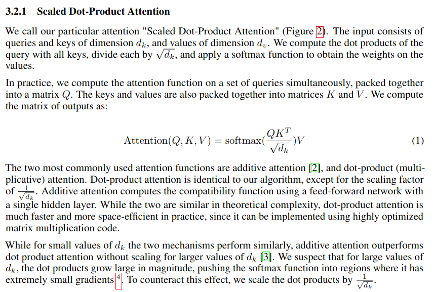
Scaling attention
# look at the paper, we implemented attention, given Q, K, V, we multiply Q and K.transpose, softmax it, then aggregating the values
# but our implementation above misses: dividing by square root of dk=head_size, so why is this done? this is called the scaled attention
# its an important normalization to have
# problem: if you have unit gaussian inputs, i.e. 0 mean, unit variance, K and Q are unit gaussian
# then if you compute 'wei' naively, then the variance will be on the order of head_size,
# but if you divide by square root of head_size, then variance will be 1, so it will be preserved
# why is this important? # scaling is used (divide by square root of head_size) to control variance at initialization
# remember that wei will feed into softmax, and its really important specially at initialization, that wei be fairly diffused
k = torch.randn(B, T, head_size)
q = torch.randn(B, T, head_size)
# wei = q @ k.transpose(-2, -1)
wei = q @ k.transpose(-2, -1) * head_size ** -0.5k.var()tensor(1.0966)q.var()
# notice the change in output here in 2 different casestensor(0.9416)wei.var()tensor(1.0065)torch.softmax(torch.tensor([0.1, -0.2, 0.3, -0.2, 0.5]), dim=-1)tensor([0.1925, 0.1426, 0.2351, 0.1426, 0.2872])torch.softmax(torch.tensor([0.1, -0.2, 0.3, -0.2, 0.5]) * 8, dim=-1)
# note: notice that the numbers move towards the max
# and we don't want these values to be too extreme, specially during initialization
# otherwise softmax will peak a lot
# so, scaling is used (divide by square root of head_size) to control variance at initializationtensor([0.0326, 0.0030, 0.1615, 0.0030, 0.8000])# modified v2.py in vscode, training there# version 4: self-attention
torch.manual_seed(1337)
B, T, C = 4, 8, 32
x = torch.randn(B, T, C)
head_size = 16
# Three linear projections: key, query, value.
key = nn.Linear(C, head_size, bias=False)
query = nn.Linear(C, head_size, bias=False)
value = nn.Linear(C, head_size, bias=False)
# Forward x through the key and query projections.
# k, q : (B, T, 16)
k = key(x) # B, T, 16
q = query(x) # B, T, 16
wei = q @ k.transpose(-2, -1) # (B, T, T)
# Causal (upper-triangular) masking.
tril = torch.tril(torch.ones(T, T))
# wei = torch.zeros((T, T)) # (older, constant version — kept for reference)
wei = wei.masked_fill(tril == 0, float('-inf'))
wei = F.softmax(wei, dim=-1) # (B, T, T), rows sum to 1
v = value(x) # B, T, 16
# Weighted aggregation.
# (B, T, T) @ (B, T, 16) -> (B, T, 16)
out = wei @ v # B, T, 16
out.shape # torch.Size([4, 8, 16])torch.Size([4, 8, 16])Multi-head attention and transformer components
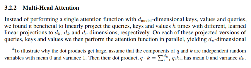
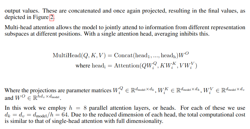
# just apply multiple attentions in parallel, and concatenating their results# deep neural nets suffer from optimization issues
# 2 optimizations dramatically help with depth of the network
# 1. SKIP connections / RESIDUAL connections (come from an old paper 2015)
# skip a connection with addition from the previous features
# addition distributes gradients equally to both of its branches
# gradients from loss hop through every addition node all the way to the input and also fork off to the residual blocks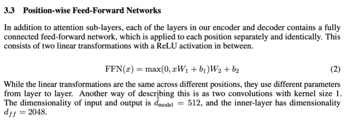
# according to this,
# dimensionality of input and output = 512
# dimensionality of inner layer = 2048
# this is 4x
# so we need to multiply the inner layer of feed forward network by 4 in our code in terms of channel sizes
# made change inside class FeedForward, 4 * n_embd
# second method
# remember that "Add & Norm" part in transformer block
# the "Add" refers to the residual part
# the "Norm" refers to the Layer Norm, and it is implemented in pytorch# LayerNorm is very similar to batchnorm (makemore series part 3)
# across the batch dimension, any individual neuron had unit gaussian distribution i.e. 0 mean, unit s.d. outputNormalization and the decoder
class BatchNorm1d:

    def __init__(self, dim, eps=1e-5, momentum = 0.1):
        self.eps = eps
        self.momentum = momentum
        self.training = True

        # parameters(trained with backprop)
        self.gamma = torch.ones(dim)
        self.beta = torch.zeros(dim)

        # buffers (trained with a running 'momentum update')
        self.running_mean = torch.zeros(dim)
        self.running_var = torch.ones(dim)

    def __call__(self, x):

        # calculate the forward pass
        if self.training:
            xmean = x.mean(0, keepdim=True) #batch mean
            xvar = x.var(0, keepdim=True, unbiased=True) #batch variance
        else:
            xmean = self.running_mean
            xvar = self.running_var

        xhat = (x - xmean) / torch.sqrt(xvar + self.eps) #normalize to unit variance
        self.out = self.gamma * xhat + self.beta

        # update the buffers
        if self.training:
            with torch.no_grad():
                self.running_mean = (1 - self.momentum) * self.running_mean + self.momentum * xmean
                self.running_var = (1 - self.momentum) * self.running_var + self.momentum * xvar
        return self.out

    def parameters(self):
        return [self.gamma, self.beta]

torch.manual_seed(1337)
module = BatchNorm1d(100)
x = torch.randn(32, 100)
x = module(x)
x.shape
torch.Size([32, 100])x[:,0].mean(), x[:,0].std() #mean, std of one feature across all batch inputs
# it guarantees 0mean, 1s.d. for every single column, its normalizing every single column of this input(tensor(7.4506e-09), tensor(1.0000))x[0,:].mean(), x[0,:].std() #mean, std of a single input from the batch, of its features
# the rows are not normalized by default(tensor(0.0411), tensor(1.0431))# layernorm: don't normalize the columns, normalize the rows
class LayerNorm1d:
def __init__(self, dim, eps=1e-5, momentum = 0.1):
self.eps = eps
self.gamma = torch.ones(dim)
self.beta = torch.zeros(dim)
def __call__(self, x):
# calculate the forward pass
xmean = x.mean(1, keepdim=True) #batch mean
xvar = x.var(1, keepdim=True, unbiased=True) #batch variance
xhat = (x - xmean) / torch.sqrt(xvar + self.eps) #normalize to unit variance
self.out = self.gamma * xhat + self.beta
return self.out
def parameters(self):
return [self.gamma, self.beta]
torch.manual_seed(1337)
module = LayerNorm1d(100)
x = torch.randn(32, 100)
x = module(x)
x.shapetorch.Size([32, 100])# the block of code is identical to the code here at pytorch:
https://docs.pytorch.org/docs/2.14/generated/torch.nn.LayerNorm.htmlx[:,0].mean(), x[:,0].std()
# the columns are not normalized by default(tensor(0.1469), tensor(0.8803))x[0,:].mean(), x[0,:].std()
# it guarantees 0mean, 1s.d. for every single row, its normalizing every single row of this input(tensor(-9.5367e-09), tensor(1.0000))# for every individual example, its 100 dimensional vector is normalized# note: few details of transformers have changed in the past years
# departs from the paper
# in paper: add and norm is applied after transformation(masked multi-head attention)
# but now its common to add and norm before transformation
# its called pre-norm formulation# dropout comes from another paper
# in neural net, it randomly every forward/backward pass, it shuts off some subset of neurons
# i.e. randomly drops some neurons to zero and trains without them
# what this does is because the mask of what is dropped out changes every single forward/backward pass
# it ends up training an ensemble of sub networks
# and at test time, everything is fully enabled and those sub networks are merged into a single ensemble
# simply: it is a regularization technique
# we added it cuz we want to scale our model a little bit, and were concerned about overfitting# we successfully implemented a decoder only transformer# there's no encoder part of the classic 'attention is all you need's block diagrams encoder section'
# no cross attention
# and the reason we're not using those is cuz we're only generating text
# the original paper was concerned with translating eg. a sentence in french to english